gkyl Tools
Tools are pre-packaged programs that are often useful but not part of the main App system. For example, there are tools to run and query the the regression test system and its output, solve the exact Reimann problem for the Euler equations and compute linear dispersion solvers for multi-moment multifluid equations, and coming soon, linear dispersion solvers for kinetic equations.
To get a list of all the supported tools do:
gkyl -t
This will give the list of tools and provide a one-line description of what the tool does. Each tool comes with its own embedded help system. For example, to see how to run the exact Euler Reimann solver tool do:
gkyl exacteulerrp -h
This will print the help and the command options for the tool to the terminal.
On this page the main tools are documented.
Solving the exact Reimann problem for Euler equations: exacteulerrp
The Reimann problem is a fundamental problem in the theory of
hyperbolic PDEs (like Euler and ideal MHD equations) which brings out
the essential nonlinear structure of the underlying physics. In
particular, the solution to the Reimann problem shows the shocks,
contact discontinuities and rarefactions waves supported by a system
of hyperbolic equations. The exacteulerrp solves the Reimann
problem exactly for the 1D Euler equations
where
is the total energy contained in the fluid. To get help for this tool do:
gkyl exacteulerrp -h
Note that the exacteulerrp tool itself can print an example input
file to shell that you can then redirect to a file
gkyl exacteulerrp -e > sod-shock.lua
To run this tool make an input file (or modify the one produced by the -e option) with the left and right initial states, the time to compute the solution at and a grid resolution. (The grid is used to determine where the solution is computed. The solution at each grid location is exact and does not depend on the resolution).
lower = -1.0 -- left-edge of domain
upper = 1.0 -- right-edge of domain
location = 0.0 -- location of shock
ncell = 100 -- Number of cells to use
tEnd = 0.2 -- Time at which to compute RP
gasGamma = 1.4 -- Gas adiabatic index

-- left/right states { density, velocity, pressure }
leftState = { 1.0, 0.0, 1.0 }
rightState = { 0.125, 0.0, 0.1 }
If this file was saved as “sod-shock.lua” you can run the tool:
gkyl exacteulerrp -i sod-shock.lua
This will produce a set of BP files with the solution to the Riemann problem:
sod-shock_density.bp          sod-shock_pressure.bp
sod-shock_internalenergy.bp   sod-shock_velocity.bp
You can now use postgkyl to plot the solution. For example, to plot all the files in a single figure do:
pgkyl "sod-shock_*.bp" pl -b
to produce the following plot.
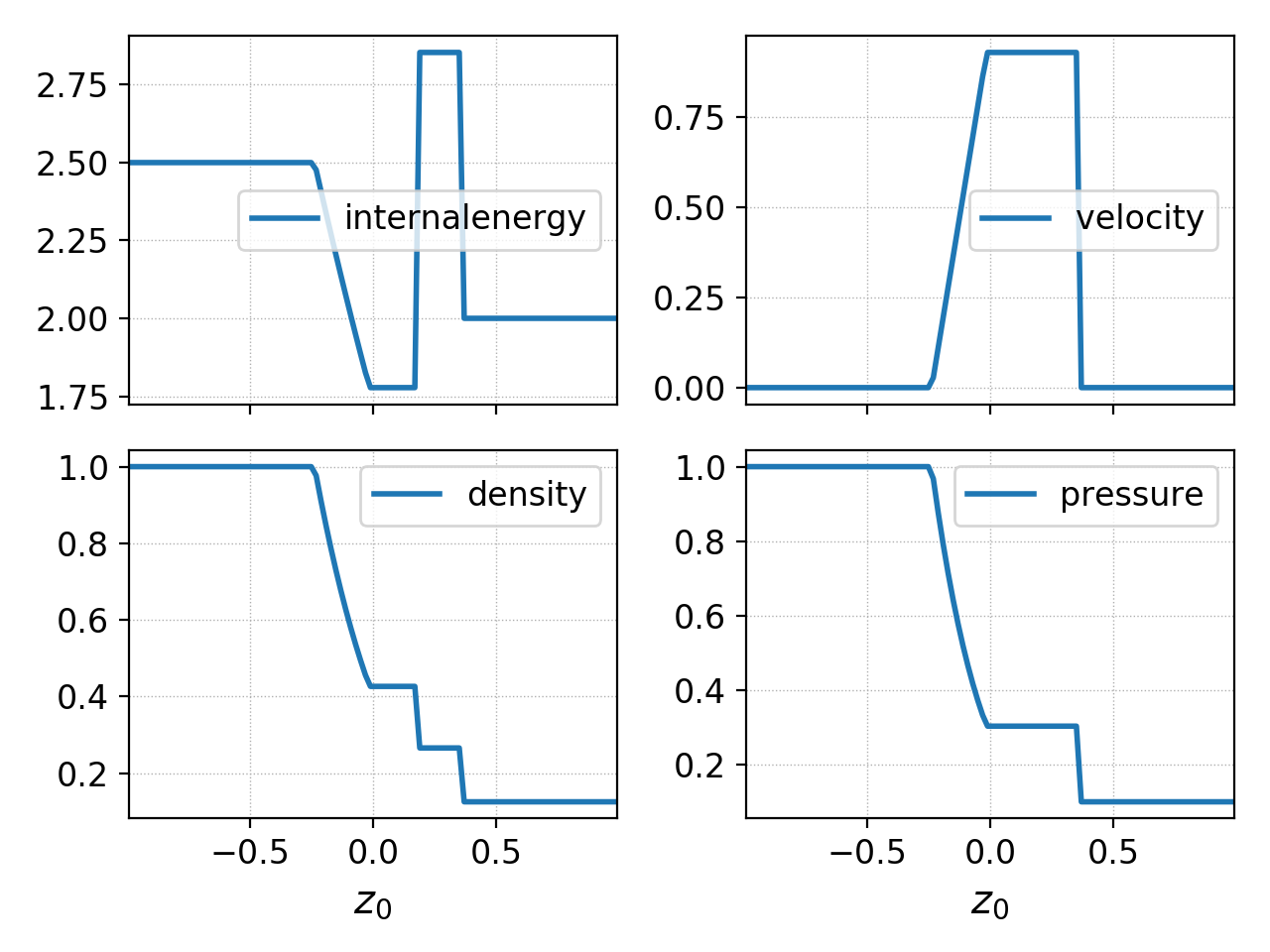
The exact solution to the sod-shock Riemann problem computed using
the exacteulerrp tool.
For a comprehensive set of 1D Riemann problems used to benchmark two finite-volume schemes see this note
Linear dispersion relation solver: multimomlinear
The multimomlinear allows solving linear dispersion equations for
multi-moment multifluid equations and will eventually be extended to
full kinetic equations. This tool allows arbitrary number of species,
each of which can be either an isothermal fluid, a five-moment fluid
or a ten-moment fluid. The fields can be computed from Maxwell
equations or Poisson equations, with the option of some species
“ignoring” the background fields. Certain forms of closures, including
non-local Hammett-Perkins Landau fluid closures, can be used.
For the list of equations and a brief overview of the algorithm used, please see this technical note. Essentially, the key idea of this algorithm is to convert the problem of finding the dispersion relation to an eigenvalue problem and then use a standard linear algebra package (Eigen in this case) to compute the eigensystem. This allows great flexibility as there is no need to directly find complex nonlinear polynomial roots or even formulate the dispersion relation explicitly.
A more careful set of benchmarks and applications are presented in this document.
To run this tool prepare an input file with the species you wish to include, the field and the set of wave-numbers at which the dispersion relation should be computed. An example input file for cold electron and ions is given below.
local Species = require "Tool.LinearSpecies"

-- Electrons
elc = Species.Isothermal {
   mass = 1.0, -- mass
   charge = -1.0, -- charge
   density = 1.0, -- number density
   velocity = {0.0, 0.0, 0.0}, -- velocity vector
   temperature = 0.0, -- temperature
}

-- Ions
ion = Species.Isothermal {
   mass = 25.0, -- mass
   charge = 1.0, -- charge
   density = 1.0, -- number density
   velocity = {0.0, 0.0, 0.0}, -- velocity vector
   temperature = 0.0, -- temperature
}

-- EM field
field = Species.Maxwell {
   epsilon0 = 1.0, mu0 = 1.0,

   electricField = {0.0, 0.0, 0.0}, -- background electric field
   magneticField = {1.0, 0.0, 0.75}, -- background magnetic field
}

-- list of species to include in dispersion relation
speciesList = { elc, ion }

-- List of wave-vectors for which to compute dispersion relation
kvectors = {}

local kcurr, kmax, NK = 0.0, 4.0, 401
dk = (kmax-kcurr)/(NK-1)
for i = 1, NK do
   kvectors[i] = {kcurr, 0.0, 0.0} -- each k-vector is 3D
   kcurr = kcurr + dk
end
Any number of species can be specified and the field can be either
Species.Maxwell or Species.Poisson. The wave-vectors at which
to compute the dispersion are specified in the kvector table,
which is a list of three element tables (with components \(k_x,
k_y, k_z\)).
To run this input file (say it is saved in cold-plasma.lua):
gkyl multimomlinear -i cold-plasma.lua
This will create a output file named cold-plasma_frequencies.bp, with the eigenvalues stored in a Gkeyll “DynVector” object.
For each element in the dynvector, the first three components are the components of the wave-vector and the rest the corresponding \(\omega_n(\mathbf{k})\) with real and imaginary parts stored separately (next to each other). You can plot the real part of the frequencies as function of wave-vector (say \(k_x\)) as:
pgkyl cold-plasma_frequencies.bp val2coord -x0 -y 3::2 pl -s -f0 --xlabel "k" --ylabel '$\omega_r$' --markersize=2
And the imaginary parts as:
pgkyl cold-plasma_frequencies.bp val2coord -x0 -y 4::2 pl -s -f0 --xlabel "k" --ylabel '$\omega_r$' --markersize=2
Often, it is useful to plot the eigenvalues in the complex plane (real part on X-axis and imaginary part on the Y-axis). For this do:
pgkyl cold-plasma_frequencies.bp val2coord -x3::2 -y 4::2 pl -s -f0 --xlabel '$\omega_r$' --ylabel '$\omega_i$' --markersize=2
Note that the frequencies are not outputed in any particular
order. Hence it is not possible to easily extract a single “branch” of
the dispersion relation from the output. Please see pgkyl help to
understand what the val2coord and pl (short for plot) do
and how to use them.
Example of the real frequency for the cold plasma waves is shown below
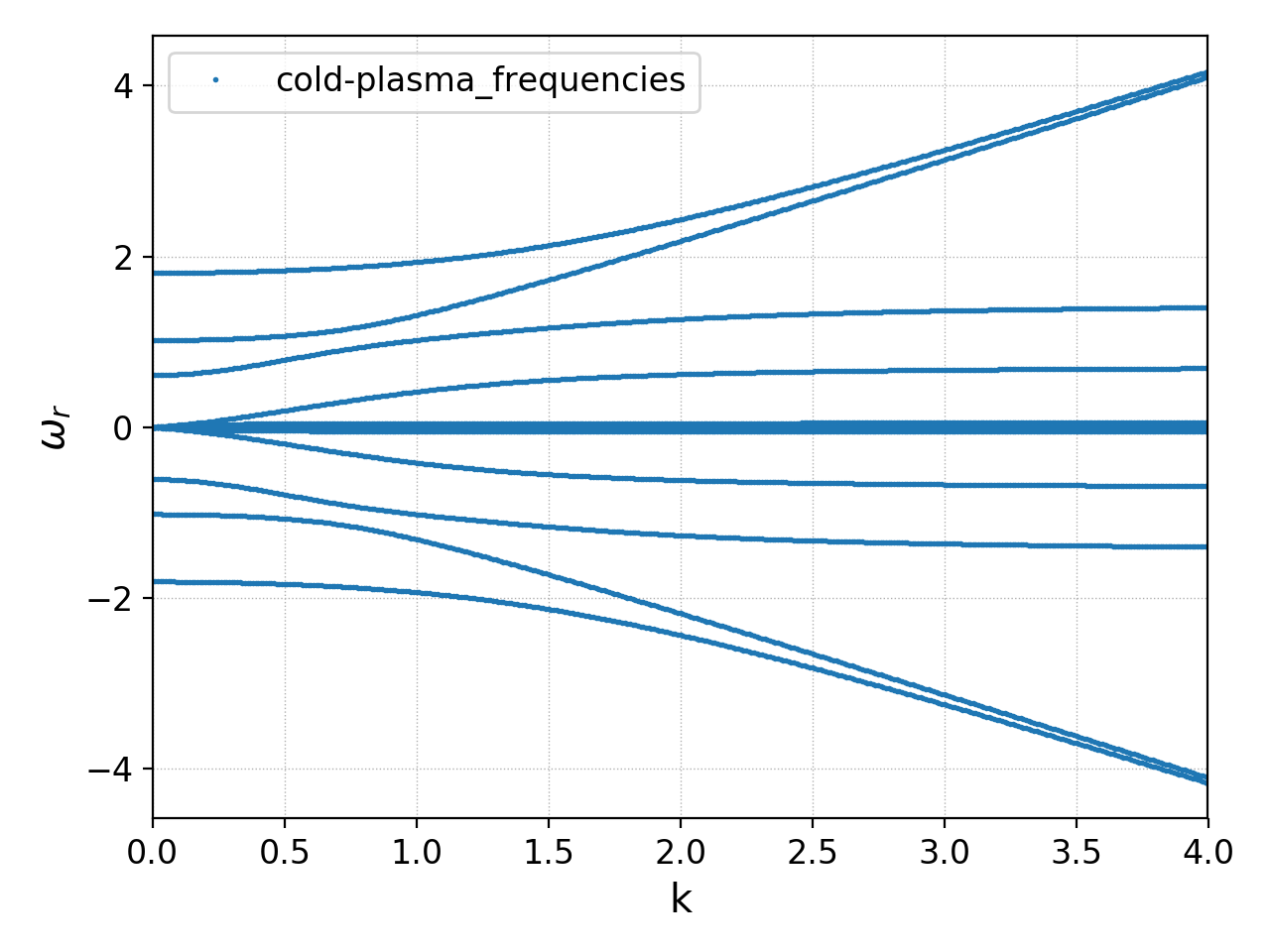
Cold plasma dispersion computed using multimomlinear tool. Seen
are the L-mode branch, the two branches of the R-mode, and the
low-frequency ion-scale waves.
The species objects can be one of Species.Isothermal,
Species.Euler or Species.Tenmoment. The input parameters
accepted by each of these objects are given below. Note that the input
parameters can either be dimensional or dimensionless. The tool itself
does not use any non-dimensionalization.
The Species.Isothermal takes the following parameters:
Parameter |
Description |
Default |
|---|---|---|
mass |
Mass of particle |
|
charge |
Charge on particle |
|
density |
Number density |
|
velocity |
Velocity vector {\(v_x\), \(v_y\), \(v_z\)} |
|
temperature |
Fluid temperature (set to zero for cold fluid) |
|
ignoreBackgroundField |
Do not consider background electromagnetic field on species. |
false |
The Species.Euler takes the following parameters:
Parameter |
Description |
Default |
|---|---|---|
mass |
Mass of particle |
|
charge |
Charge on particle |
|
density |
Number density |
|
velocity |
Velocity vector {\(v_x\), \(v_y\), \(v_z\)} |
|
pressure |
Fluid pressure |
|
gasGamma |
Gas adiabatic index |
5/3 |
ignoreBackgroundField |
Do not consider background electromagnetic field on species. |
false |
The Species.Tenmoment takes the following parameters:
Parameter |
Description |
Default |
|---|---|---|
mass |
Mass of particle |
|
charge |
Charge on particle |
|
density |
Number density |
|
velocity |
Velocity vector {\(v_x\), \(v_y\), \(v_z\)} |
|
pressureTensor |
Pressure in the fluid frame as a table {\(P_{xx}\), \(P_{xy}\), \(P_{xz}\), \(P_{yy}\), \(P_{yz}\), \(P_{zz}\)} |
|
useClosure |
Flag to turn on various collisionless closures |
|
chi |
Multiplicative factor in closure. |
\(\sqrt{4/9\pi}\). |
ignoreBackgroundField |
Do not consider background electromagnetic field on species. |
false |
Note
Presently, a unmagnetized Hammett-Perkins closure is implemented. See tech-note linked above and [Ng2017]. This is not always very useful and accurate, specially for strongly magnetized problems. We hope to implement better closures soon.
The
ignoreBackgroundFieldallows a species to “ignore” the applied background electromagnetic fields. This is often useful when one species is unmagnetized.
References
J. Ng, A. Hakim, A. Bhattacharjee, A. Stanier, & W. Daughton “Simulations of anti-parallel reconnection using a nonlocal heat flux closure”. Physics of Plasmas, 24 (8), 082112–5. (2017) http://doi.org/10.1063/1.4993195