collect¶

Assemble multiple active datasets into a new, single dataset.

It is also possible to collect datasets into chunks (multiple datasets) of a specified size rather than into a single dataset.

Command line¶

pgkyl collect --help
  Usage: pgkyl collect [OPTIONS]

    Collect data from the active datasets and create a new combined dataset.
      The time-stamp in each of the active datasets is collected and used as the
      new X-axis. Data can be collected in chunks, in which case several
      datasets are created, each with the chunk-sized pieces collected into each
      new dataset.

    Options:
      -s, --sumdata        Sum data in the collected datasets (retain components)
      -p, --period FLOAT   Specify a period to create epoch data instead of time
                           data

      --offset FLOAT       Specify an offset to create epoch data instead of time
                           data  [default: 0.0]

      -c, --chunk INTEGER  Collect into chunks with specified length rather than
                           into a single dataset

      -u, --use TEXT       Specify a 'tag' to apply to (default all tags).
      -t, --tag TEXT       Specify a 'tag' for the result.
      -l, --label TEXT     Specify the custom label for the result.
      -h, --help           Show this message and exit.

There are many uses of the collect command. One such use, for example, is to plot quantities over time. If we consider the two stream instability Vlasov-Maxwell simulation we can gather the \(x\)-component of the electric field from all frames and plot it as a function of time and space with

pgkyl "two-stream_field_[0-9]*.bp" interp sel -c0 collect pl -x 'time' -y 'x'

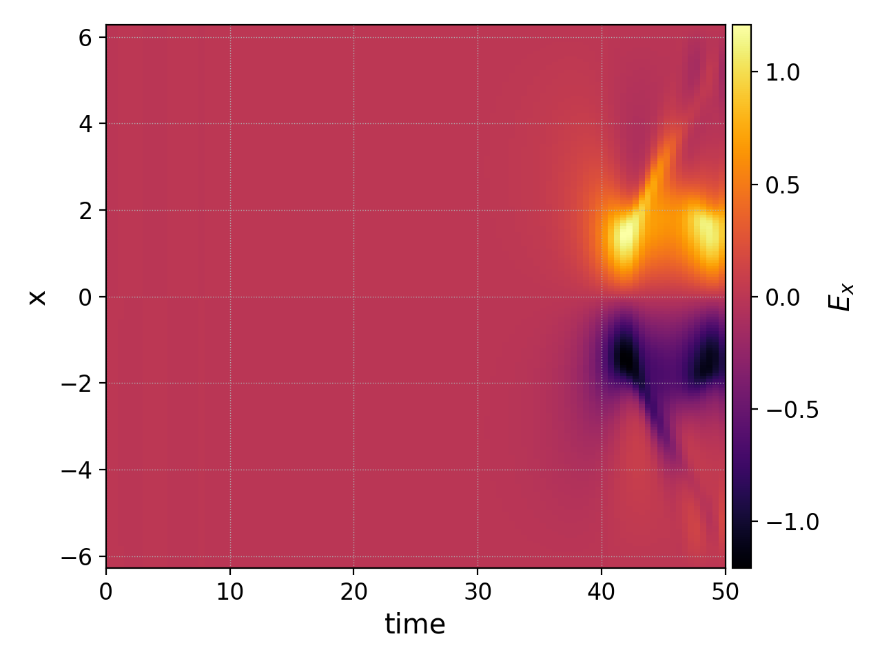
The field is very small at first but is exponentially growing, so in the above figure we mostly see the saturated electric field at later times.

The collect command is also able to collect datasets into chunks of a specified length with the -c flag. So suppose we wish to compute a time average of the electric field over three separate periods in the two stream instability simulation (we will set nFrame=98 in the gkyl input file for this example so there are a total of 99 frames), we can collect the field data into three separate datasets with 33 frames each and use the ev command to average in time (0th dimension) as follows:

pgkyl "two-stream_field_[0-9]*.bp" interp sel -c0 collect -c 33 ev -l 'frames 0-32' 'f[99] 0 avg' \
  ev -l 'frames 33-65' 'f[100] 0 avg' ev -l 'frames 66-98' 'f[101] 0 avg' activ -i102:105 \
  pl -x '$x$' -y '$\langle E_x\rangle_t$'

producing the following three plots

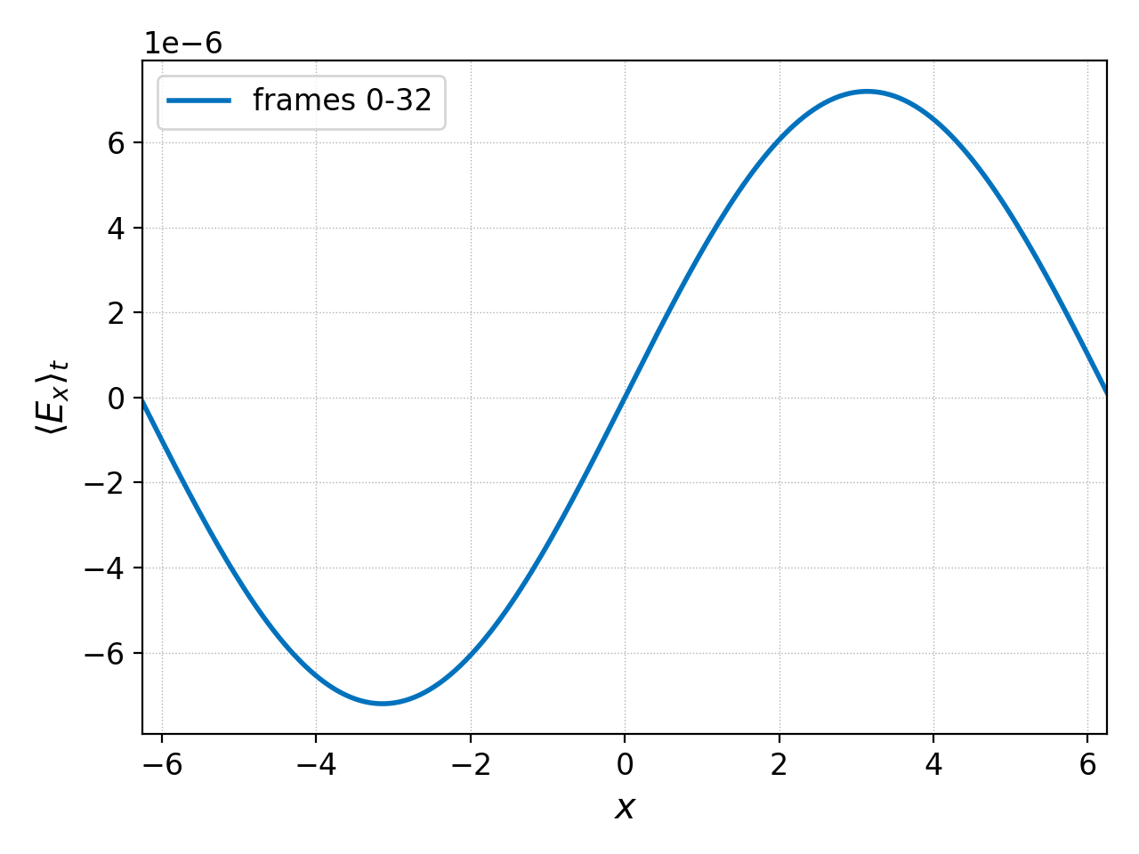
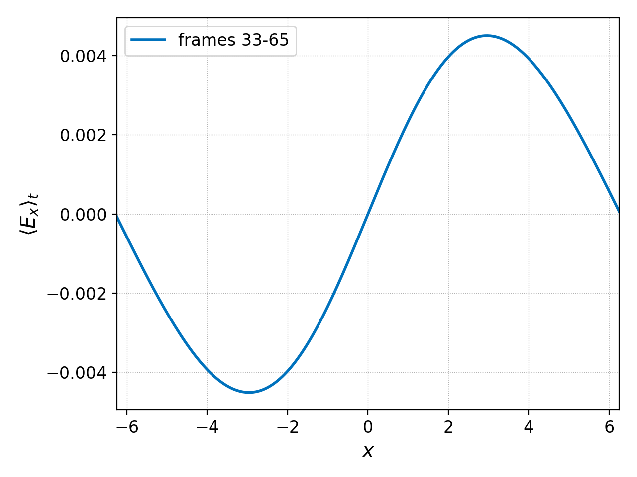
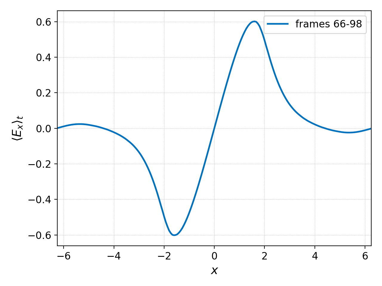
Clearly the field amplitude averaged over 30 frame intervals is increasing as the instability develops.

Finally, collect allows a transformation of the time dimension so that instead of time t it instead becomes (t-offset)/period via the --offset and --period flags. This is used, for example, in astronomy for variable stars and in creating Poincare plots (see http://ammar-hakim.org/sj/je/je32/je32-vlasov-test-ptcl.html).