differentiate¶

Compute the derivatives of a function along each direction. This returns a dataset with as many components as there are dimensions in the original dataset, i.e. it returns the gradient, unless the -d flag is used to specify a direction.

This command takes the basis expansion in a cell, differentiates it analytically in the desired directions, and then interpolates it onto a finer mesh in the same fashion as the interpolate command.

Note that differentiation is also possible with the ev command and the grad operation.

Command line¶

pgkyl differentiate -h
  Usage: pgkyl differentiate [OPTIONS]

    Interpolate a derivative of DG data on a uniform mesh

  Options:
    -b, --basistype [ms|ns|mo]  Specify DG basis
    -p, --polyorder INTEGER     Specify polynomial order
    -i, --interp INTEGER        Interpolation onto a general mesh of specified
                                amount

    -d, --direction INTEGER     Direction of the derivative (default: calculate
                                all)

    -r, --read BOOLEAN          Read from general interpolation file
    -t, --tag TEXT              Specify a 'tag' to apply to (default all tags).
    -o, --outtag TEXT           Optional tag for the resulting array
    -h, --help                  Show this message and exit.

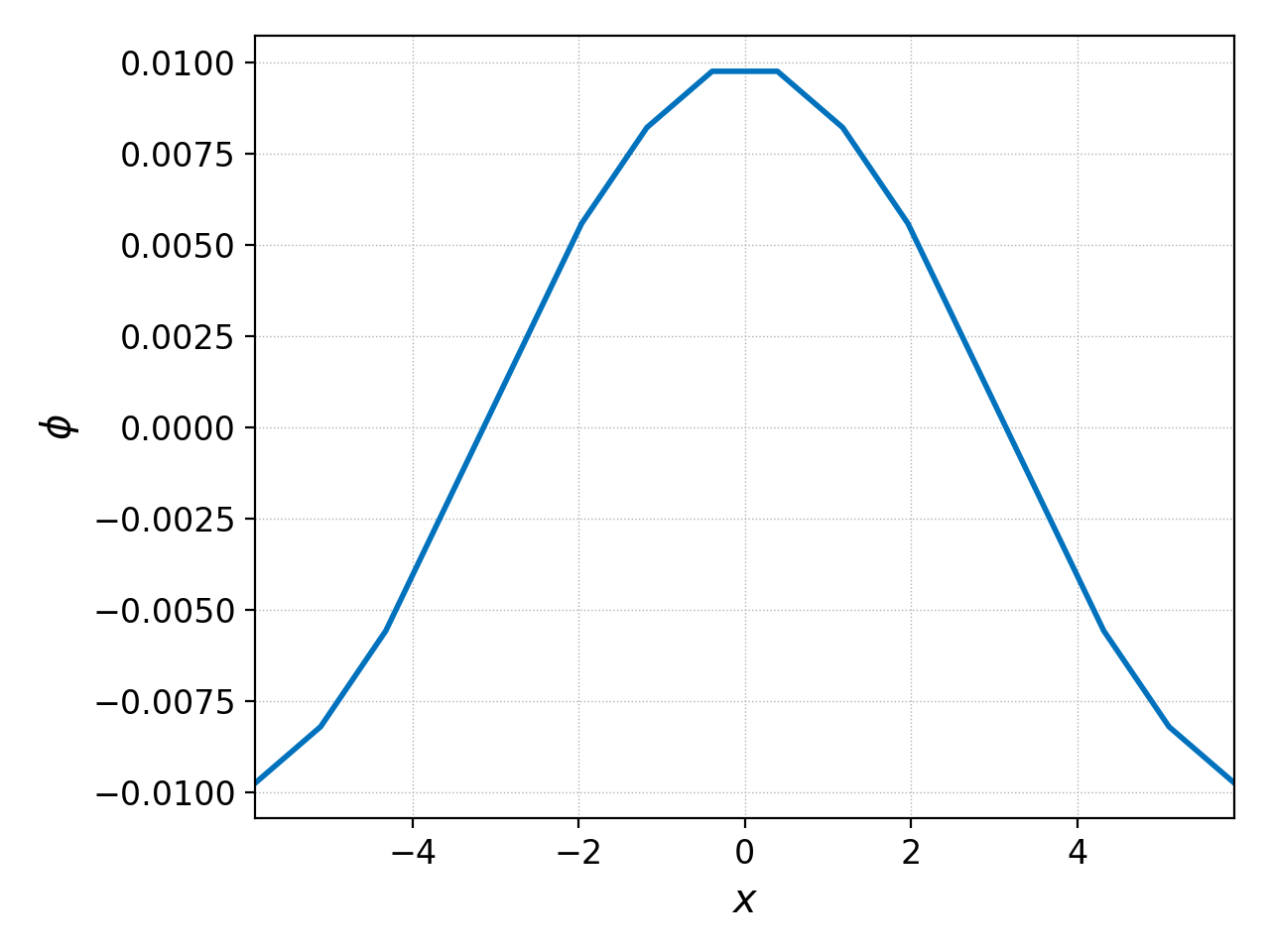
Let’s take a gyrokinetic ion acoustic wave simulation as an example. We can examine the initial electrostatic potential generated by the initial conditions with

pgkyl gk-ionSound-1x2v-p1_phi_0.bp interp pl -x '$x$' -y '$\phi$'

giving the plot shown below on the left.

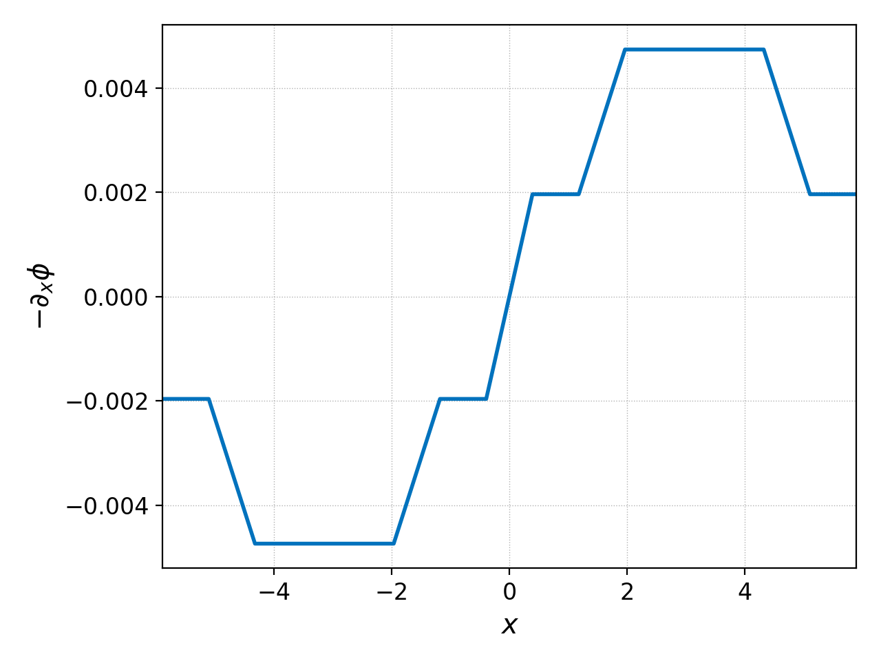
Suppose we wished to know what the initial electric field is, then we would differentiate the potential and multiply it by -1 as follows

pgkyl gk-ionSound-1x2v-p1_phi_0.bp diff -d 0 ev 'f[1] -1 *' pl -x '$x$' -y '$-\partial_x\phi$'

Note we we have abbreviated differentiate -> diff, either is allowed. This command produces the electric field above on the right. It is cellwise constant because we use a piecewise linear basis function.

Now suppose you wish to examine the gradient of the ion distribution function at \(t=0\) and \(x=0\). This can be accomplished with the following command

pgkyl gk-ionSound-1x2v-p1_ion_0.bp diff sel --z0 0. pl -x '$v_\parallel$' -y '$\mu$'

in order to produce:

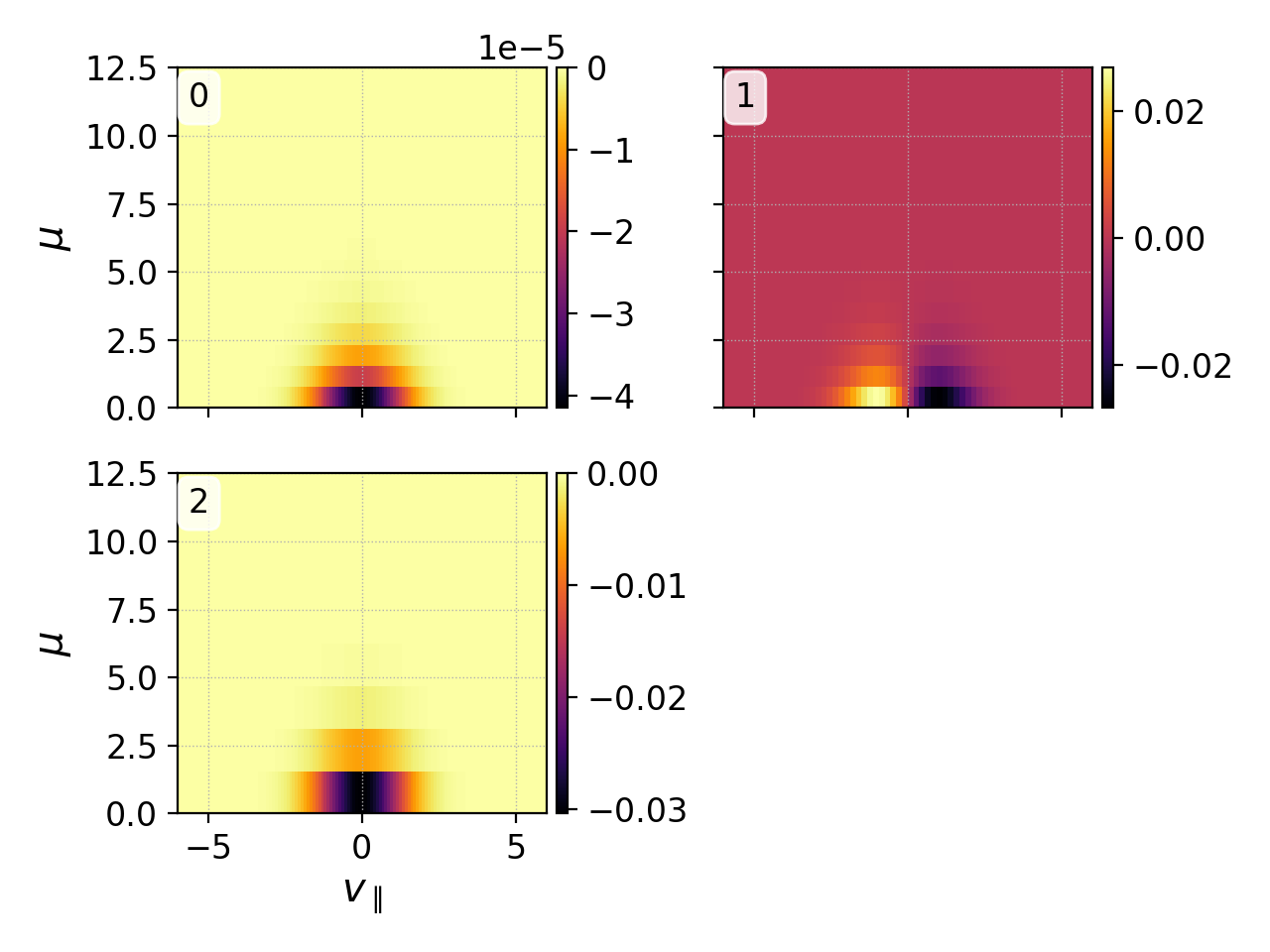
Starting with the top left and going clockwise, this plot provides the gradient in \(f_i(x,v_\parallel,\mu)\) along \(x\), \(v_\parallel\) and \(\mu\), all three evaluated at \(x=0\).