fft¶

Command line¶

pgkyl fft --help
  Usage: pgkyl fft [OPTIONS]

    Calculate the Fourier Transform or the power-spectral density of input
    data. Only works on 1D data at present.

  Options:
    -p, --psd         Limits output to positive frequencies and returns the power
                      spectral density |FT|^2.
    -i, --iso         Bins power spectral density |FT|^2, making 1D power
                      spectra from multi-dimensional data.
    -u, --use TEXT    Specify a 'tag' to apply to (default all tags).
    -t, --tag TEXT    Optional tag for the resulting array
    -l, --label TEXT  Custom label for the result
    -h, --help        Show this message and exit.

Fourier analysis on one-dimensional data is available in pgkyl. This does not mean that the simulation has to be 1D, but for higher-D simulations one must first reduce the dimensionaly of the data before doing an FFT.

For example, we take a simple incompressible Euler 2D simulation of a velocity shear instability (Kelvin Helmholtz). Using the pgkyl command

pgkyl "incompEuler-KH-2x-p1_fluid_[0-9]*.bp" interp anim -a -x 'x' -y 'y' --clabel '$\psi(x,y)$'

we obtain the following velocity potential

This simulation was initialized with a slow variation in x and a small but more oscillatory perturbation in y:

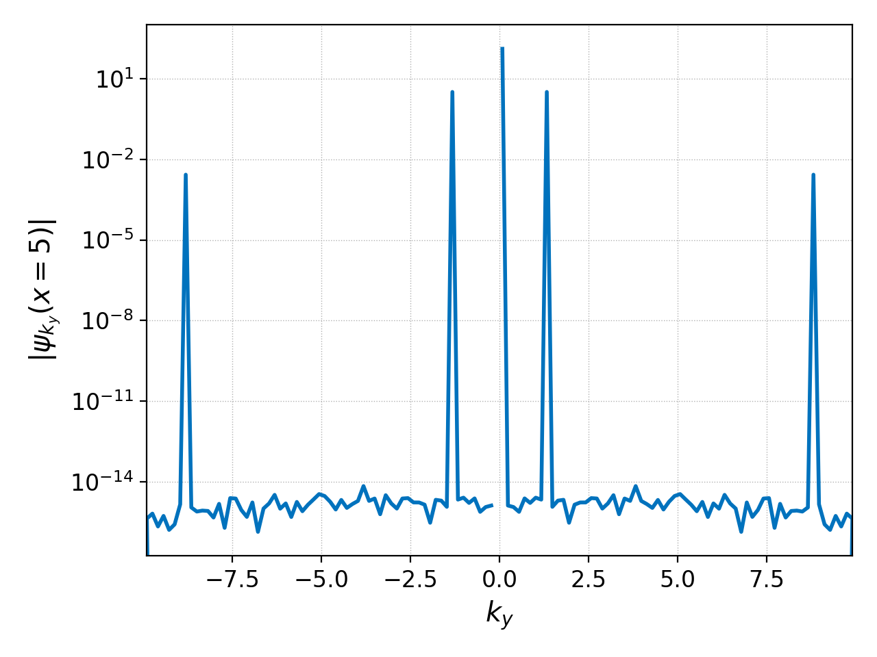
where \(\alpha=0.05\), \(k_x=2\pi/L_x\), \(k_y=16\pi/L_y\), and \(L_y=4L_x=40\). If we were to examine the Fourier transform of this initial condition at \(x=5\) with

pgkyl incompEuler-KH-2x-p1_fluid_0.bp interp sel --z0 5. fft ev 'f[0] abs' pl -x '$k_y$' -y '$\psi_{k_y}(x=5)$' --logy --xscale 6.283185

where we scaled the \(x\)-axis by \(2\pi\) because of SciPy’s fftfreq convention, we would obtain

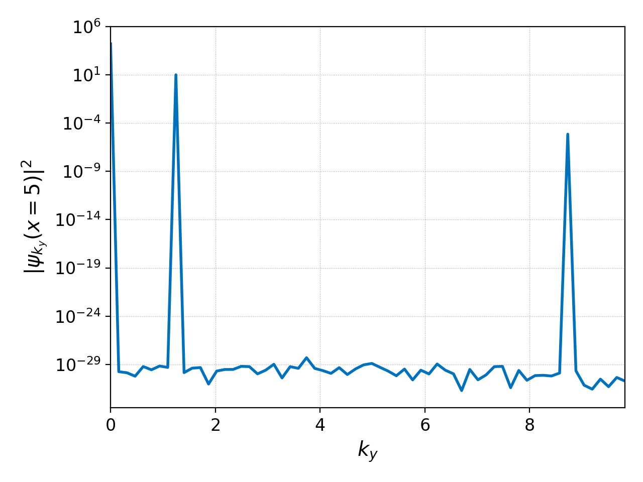
or most commonly one looks at the power spectrum of a signal, which we can obtain with the -p flag:

pgkyl incompEuler-KH-2x-p1_fluid_0.bp interp sel --z0 5. fft -p pl -x '$k_y$' -y '$|\psi_{k_y}(x=5)|^2$' --xscale 6.283185 --logy

This plot has the peak we would expect at \(k_y=16\pi/L_y=1.2566\), but it also has two other peaks we did not expect. This is because we are FFT-ing interpolated DG data which introduces modes if the transform is not done weakly (not covered here).

We could also look at how this spectrum changes in time with the following command

pgkyl "incompEuler-KH-2x-p1_fluid_[0-9]*.bp" interp sel --z0 5. fft -p collect pl --group 1 --logy -x '$k_y/(2\pi)$' -y '$\left|\psi_{k_y}(x=5)\right|^2$' --clabel 'time'

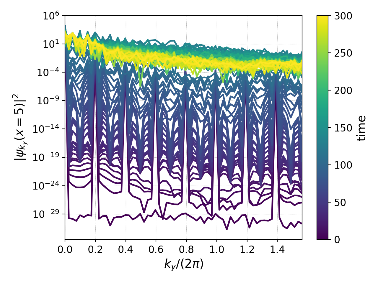
showing how the spectrum goes from being peaked at specific \(k_y\)’s to being a fully filled spectrum when turbulence sets in.

Script mode¶

Although it is possible to call postgkyl’s fft command from a script, we recommend that you instead use SciPy’s fft package directly (or alternatively NumPy’s fft package). Here’s an example of how to perform the same FFT described in the command line section above

import postgkyl as pg
from scipy.fft import fft, fftfreq
import matplotlib.pyplot as plt
import numpy as np

fileName = 'incompEuler-KH-2x-p1_fluid_0.bp'
polyOrder, basisType = 1, 'ms'

pgData   = pg.GData(fileName)
pgInterp = pg.GInterpModal(pgData, polyOrder, basisType)
pgInterp.interpolate(overwrite=True)
yInt, psi_z0eq5p0 = pg.data.select(pgData, z0=5.0)

y = 0.5*(yInt[1][:-1]+yInt[1][1:])

ky, psi_z0eq5p0_ky = 2.*np.pi*fftfreq(np.size(y)), fft(np.squeeze(psi_z0eq5p0))

plt.semilogy(ky, np.abs(psi_z0eq5p0_ky))
plt.show()

where we used the select command to pick the data at \(x=5\), transformed the \(y\) coordinates from nodal to cell-center coordinates, and squeezed the data to remove redundant dimensions.