growth¶

Measure the growth rate in the time trace of a quantity, assuming that it is a squared quantity (e.g. \(\phi^2\), \(|\mathbf{E}|^2\)). If one applies this to a non-squared quantity then the growth-rate would be off by a factor of two.

Command Docstrings

The command works by fitting \(A e^(2\gamma t)\) to the data and returning \(\gamma\).

Command line¶

Command help

 $ pgkyl growth --help
 Usage: pgkyl growth [OPTIONS]

 Attempts to compute growth rate (i.e. fit e^(2x)) from DynVector data,
 typically an integrated quantity like electric or magnetic field energy.

 Options:
   -u, --use TEXT                Specify a 'tag' to apply to (default all
                                 tags).

   -g, --guess <FLOAT FLOAT>...  Specify initial guess
   -p, --plot                    Plot the data and fit
   --minn INTEGER                Set minimal number of points to fit
   --maxn INTEGER                Set maximal number of points to fit
   -i, --instantaneous           Plot instantaneous growth rate vs time
   -h, --help                    Show this message and exit.

The two tream instability simulation produces a field energy time trace that can be plotted with

pgkyl two-stream_fieldEnergy.bp sel -c0 pl --logy

../../_images/two-stream_fieldEnergy.png

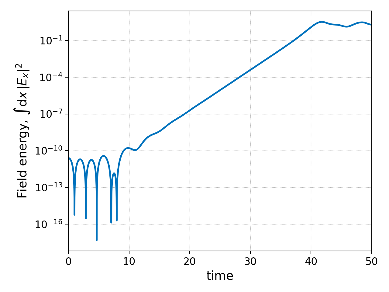
We have selected the \(E_x\) component because all other field components are essentially zero. We can then measure the growth rate in the field energy with the following command

pgkyl two-stream_fieldEnergy.bp sel -c0 growth

Such command produces the output below

fitGrowth: fitting region 100 -> 7916
gamma = +3.79836e-01 (current +5.814e-02 R^2=7.407e-01)    99.99% done [========= ]
gamma = +3.79836e-01

This output indicates that it made the measurement taking into account all the data between the 100th and the 7916th point (if you examine the file two-stram_fieldEnergy.bp you’d find that it has 7916 data points), and arrived at the growth rate \(\gamma=0.379836\), the the \(R^2\) of the fit being 0.7407.

The growth command also allows for specifying a window in which to perform the measurement via the --minn and --maxn flags. We could then limit the window between the 2000th and the 6000th point with

pgkyl two-stream_fieldEnergy.bp sel -c0 growth --minn 2000 --maxn 6000

and the output would be

fitGrowth: fitting region 2000 -> 6000
gamma = +3.79836e-01 (current +4.322e-01 R^2=9.998e-01)    99.98% done [========= ]
gamma = +3.79836e-01

giving the same result obtained above.

There is also an option for specifying a guess to \(A\) and \(\gamma\) in the fit, via the -g flag:

pgkyl two-stream_fieldEnergy.bp sel -c0 growth --minn 2000 --maxn 6000 -g 1. 0.36

fitGrowth: fitting region 2000 -> 6000
gamma = +3.79836e-01 (current +4.322e-01 R^2=9.998e-01)    99.98% done [========= ]
gamma = +3.79836e-01