interpolate

Gkeyll’s simulation may employ higher-order methods with more than one degree of freedom per cell, typically expansion coefficients or nodal values. The interpolate command interpolates this higher-order representation onto a finer mesh with more points than the number of cells in the Gkeyll simulation.

Command Docstrings

Command line

Command help

pgkyl interpolate --help
  Usage: pgkyl interp [OPTIONS]

    Interpolate DG data onto a uniform mesh.

  Options:
    -b, --basistype [ms|ns|mo|mt]  Specify DG basis.
    -p, --polyorder INTEGER        Specify polynomial order.
    -i, --interp INTEGER           Interpolation onto a general mesh of
                                   specified amount.

    -u, --use TEXT                 Specify a 'tag' to apply to (default all
                                   tags).

    -t, --tag TEXT                 Optional tag for the resulting array
    -r, --read BOOLEAN             Read from general interpolation file.
    -n, --new                      for testing purposes
    -h, --help                     Show this message and exit.

A Gkeyll simulation can have several degrees of freedom per cell. If we simply invoke the plot command we would then obtain a plot of all the coefficients in each cell. So for example, take the electron distribution function at the end of a two stream instability simulation and plot it with

pgkyl two-stream_elc_100.bp pl -x '$x$' -y '$v_x$'

we would obtain figure below on the left, with all 8 DG expansion coefficients plotted in phase space. Most commonly we are interested in plotting the actual function that the expansion coefficients represent, rather than plotting such coefficients. We can do that by interpolating onto a finer mesh with the interpolate command:

pgkyl two-stream_elc_100.bp interp pl -x '$x$' -y '$v_x$'

which results in the figure below on the right.

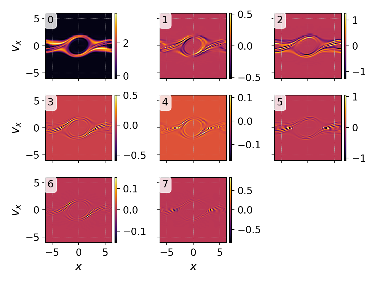
DG coefficients.

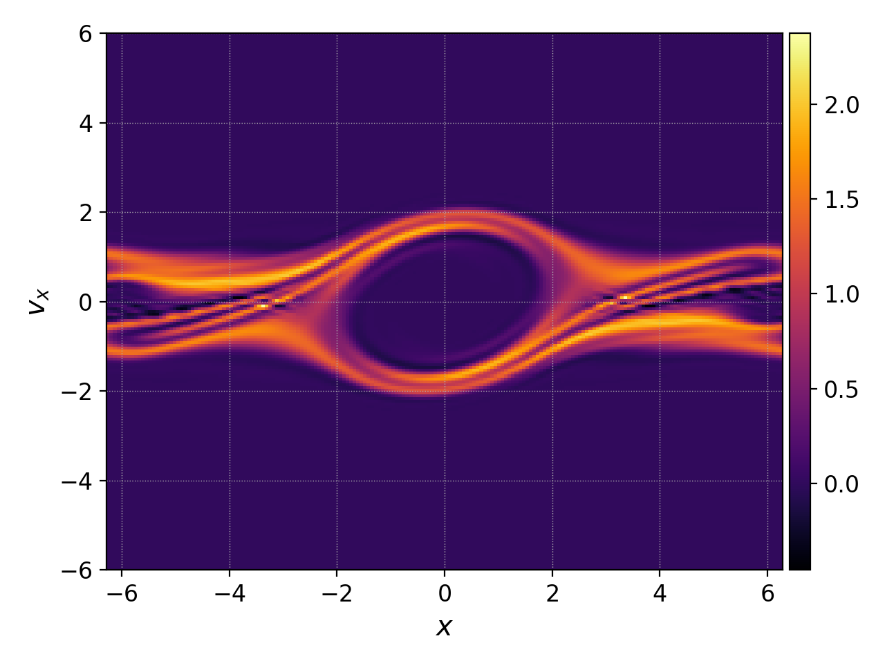
Interpolated distribution function.

We can compare the cell average of the electron distribution function with the interpolated distribution function with the following command

pgkyl two-stream_elc_100.bp -t fe interp -u fe -t fInterp sel -u fe -c0 -t c0 \
  ev -l 'cell average' -t cellAv 'c0 2 /' activ -t fInterp,cellAv pl -b

which divides the zeroth DG coefficient by 2 in order to obtain the cell average (1r 2D piecewise quadratic basis), and produces the following figure

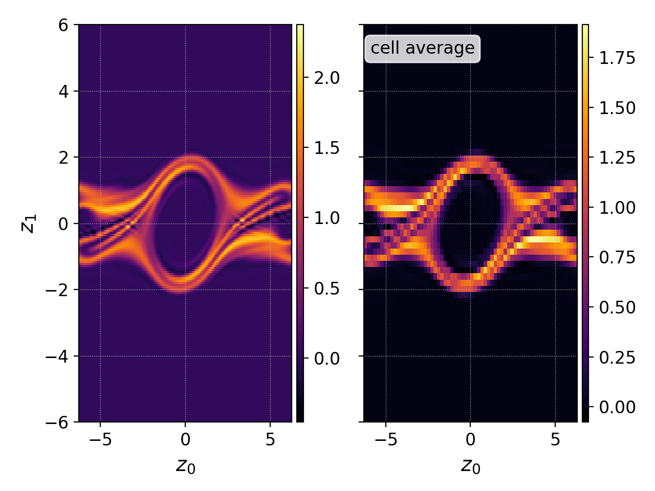
Notice how the cell average (right) is naturally coarser grained, and the interpolated function (left) offers a smoother plot.

By default the interpolate command interpolates onto a uniform mesh that subdivides each cell in the simulation into \(p+1\) cells in each direction, where \(p\) is the polynomial order of the simulation. It is also possible to interpolate onto finer meshes with the -i flag in order to obtain smoother plots. However note that interpolating onto finer meshes can also augment local maxima and/or minima. Below we compare the final electron distribution function interpolated onto a mesh with 3 subcells per cell in each direction (default for \(p=2\)) and interpolating onto a mesh with 8 subcells per cell in each direction:

pgkyl two-stream_elc_100.bp -t fe interp -t i3 interp -i 8 -u fe -t i8 activ -t i3,i8 pl -b -x '$x$' -y '$v_x$'

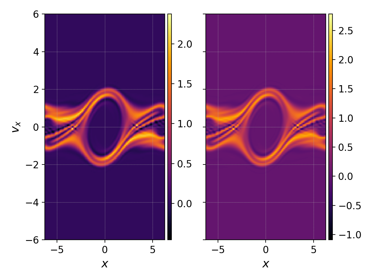
This example also shows the use of tags in order to tag datsets and to instruct interpolate which datasets to operate on (via the -u/--use flag). In order to request that interpolate operates on a given tagged dataset, one must pass -u followed by the dataset we wish to interpolate. And in order to create a new dataset outof the interpolated data one must use the -t flag followed by the name (tag) of the new dataset. In the above example the first interpolate operates on the input data (no -u necessary because it immediately precedes it and there is only one dataset at that point in the chain) and creates a dataset tagged i3. The second interpolate operates on the input data (-u fe) and creates a dataset tagged i8.

Script mode

interpolate uses the GInterpModal and GInterpNodal classes based on the DG mode.

Initialization parameters for GInterpModal and GInterpNodal

Parameter	Description	Default
gdata (GData)	A GData object to be used.
polyOrder (int)	The polynomial order of the discontinuous Galerkin discretization.
basis (str)	The polynomial basis. Currently supported options are 'ns' for nodal Serendipity, 'ms' for modal Serendipity, and 'mo' for the maximal order basis.

After the initialization, both GInterpModal and GInterpNodal can be used to interpolate data on a uniform grid and to calculate derivatives

Members of GInterpModal and GInterpNodal

Member	Description
interpolate(int component, bool stack) -> narray, narray	Interpolates the selected component (default is 0) of the DG data on a uniform grid
derivative(int component, bool stack) -> narray, narray	Calculates the derivative of the DG data

When the stack parameter is set to true (it is false by default), the grid and values are pushed to the GData stack rather than returned.

An example of the usage:

import postgkyl as pg
data = pg.data.GData('bgk_neut_0.bp')
interp = pg.data.GInterpModal(data, 2, 'ms')
iGrid, iValues = interp.interpolate()