select
Select a subset of one or multiple datasets.
This subset can can be created by
Choosing a cell along a direction (
--z#with an integer).Choosing a range of cells along a direction (
--z#with a slice).Choosing a specific component (
-c), which may be an expansion coefficient, fluid moment or, if used along with interpolate, a vector component. Multiple components can be selected with a slice of floats or with comma-separated values.Evaluating the function at a specific coordinate in one direction (using interpolate and
select --z#with a float) or segment in one dimension (using interpolate andselect --z#with a slize of floats).
Note
Postgkyl retains the number of dimensions and component index. This means that, for example, given a 16x16 2D dataset with 8 components per cell fixing the second coordinate and selecting one component will produce a dataset with a shape (16, 1, 1). For plotting purposes postgkyl treats such data as 1D.
Command line
Command help
pgkyl select --help
  Usage: pgkyl select [OPTIONS]

    Subselect data from the active dataset(s). This command allows, for
    example, to choose a specific component of a multi-component dataset,
    select a index or coordinate range. Index ranges can also be specified
    using python slice notation (start:end:stride).

  Options:
    --z0 TEXT        Indices for 0th coord (either int, float, or slice)
    --z1 TEXT        Indices for 1st coord (either int, float, or slice)
    --z2 TEXT        Indices for 2nd coord (either int, float, or slice)
    --z3 TEXT        Indices for 3rd coord (either int, float, or slice)
    --z4 TEXT        Indices for 4th coord (either int, float, or slice)
    --z5 TEXT        Indices for 5th coord (either int, float, or slice)
    -c, --comp TEXT  Indices for components (either int, slice, or coma-
                     separated)

    -u, --use TEXT   Specify a 'tag' to apply to (default all tags).
    -t, --tag TEXT   Optional tag for the resulting array
    -h, --help       Show this message and exit.
Perhaps the two most common uses of select are to choose a vector
component or to evaluate a function at a specific coordinate. Consider
the data produced by a
two stream instability Vlasov-Maxwell simulation.
The file two-stream_field_0.bp contains 24 components per cell.
That is because it contains 8 vector components (3 components of the
electric and magnetic fields each and 2 correction potentials, see
http://ammar-hakim.org/sj/maxwell-eigensystem.html) and 3
degrees of freedom per component (for piecewise linear basis in 1D).
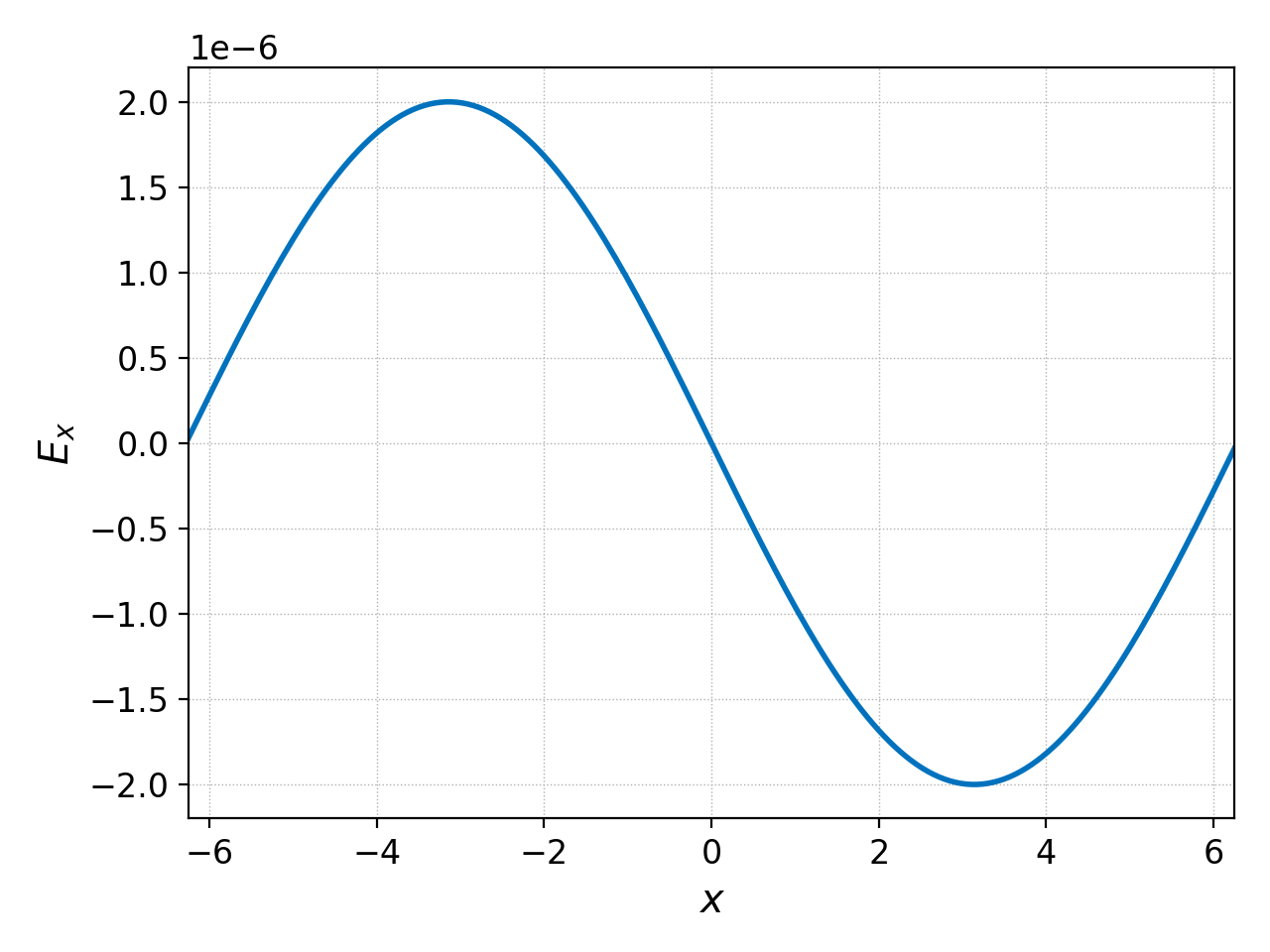
If we wish to only see \(E_x\) then we can select it and plot it
with
pgkyl two-stream_field_0.bp interp select -c0 pl
which yields the following figure
We could also select multiple components with a comma-separated list
pgkyl two-stream_field_0.bp interp select -c0,3 pl -x '$x$'
which yields the following plot of \(E_x\) and \(B_x\)
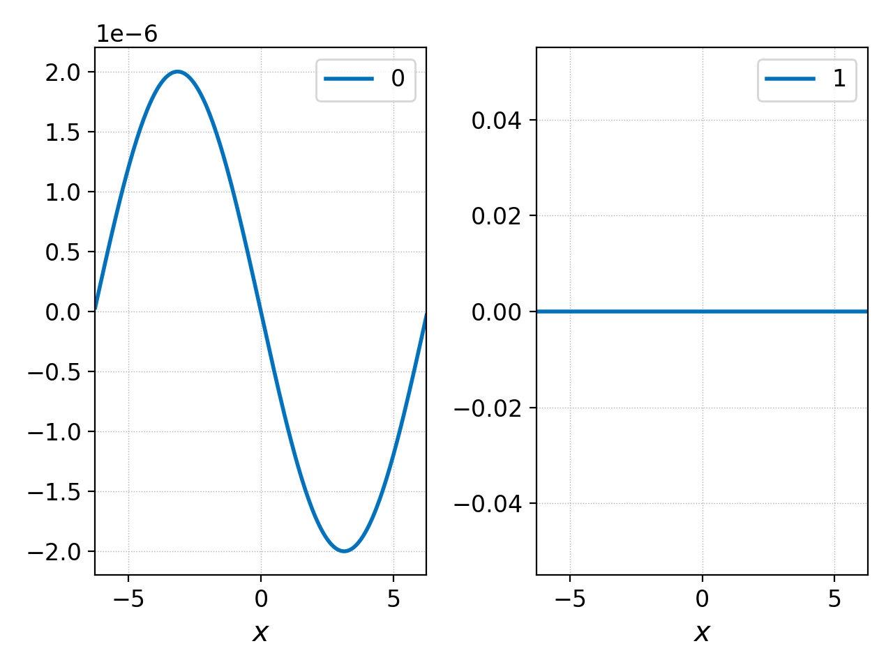
x-component of the electric and magnetic fields.
Or we could select all the components of the magnetic field in all frames with
pgkyl "two-stream_field_[0-9]*.bp" interp select -c3:6 pl -f0 -x '$x$' --no-legend --nsubplotrow 1
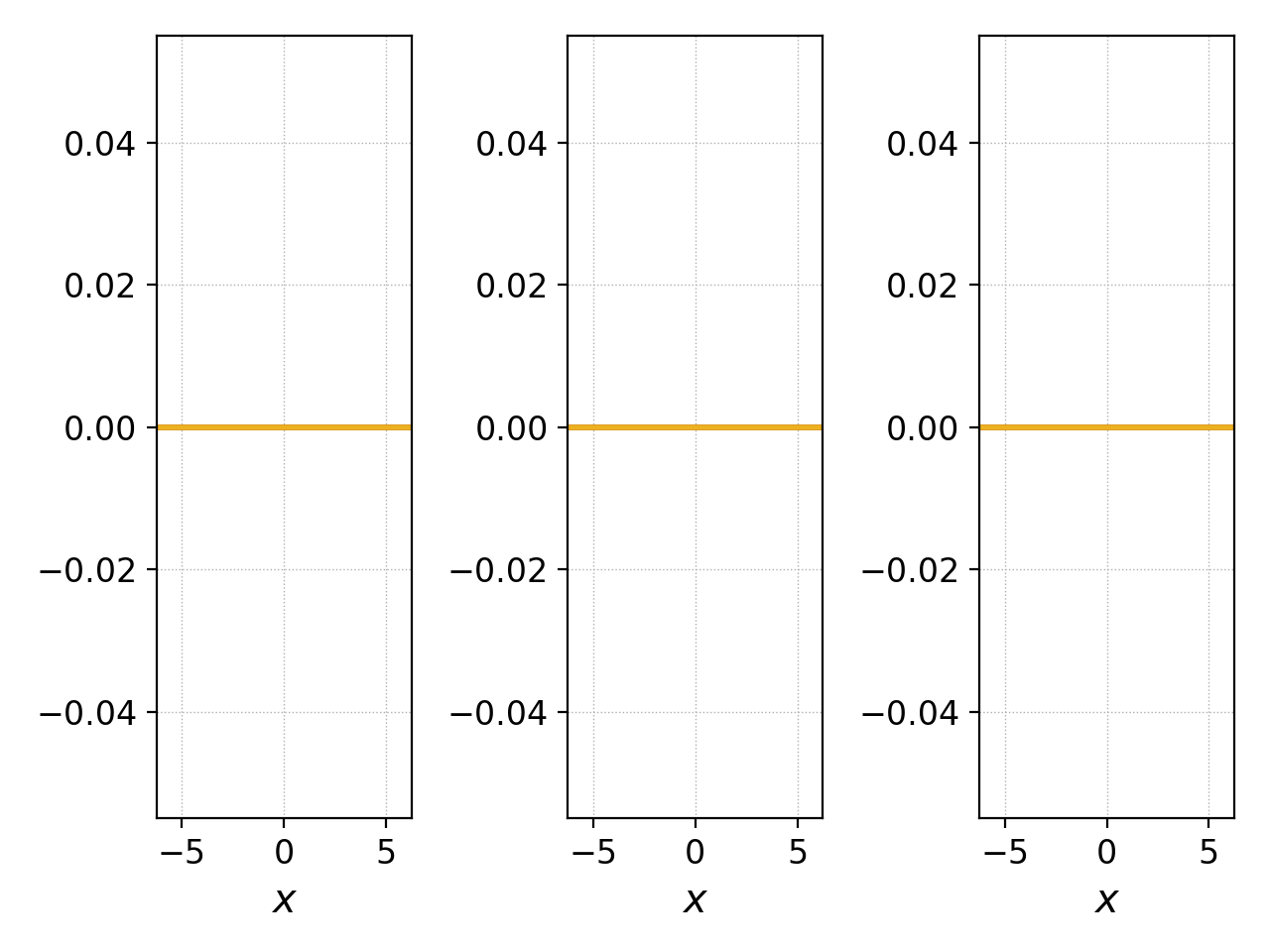
Components of the magnetic field.
to show that this is an electrostatic simulation.
As a demonstration of using select to evaluate functions at a given
coordinate we could evaluate the above \(E_x\) at \(x=-\pi\), but
that would yield a single number. We could instead load all the field
data files, evaluate the \(x\)-component of the electric field
at \(x=-\pi\) in each frame, collect all those points into a single
dataset, and plot them as a function of time. This would be accomplished
with the following command
pgkyl "two-stream_field_[0-9]*.bp" interp sel -c0 --z0 -3.14159 collect pl -x 'time' -y '$E_x(x=-\pi,t)$'
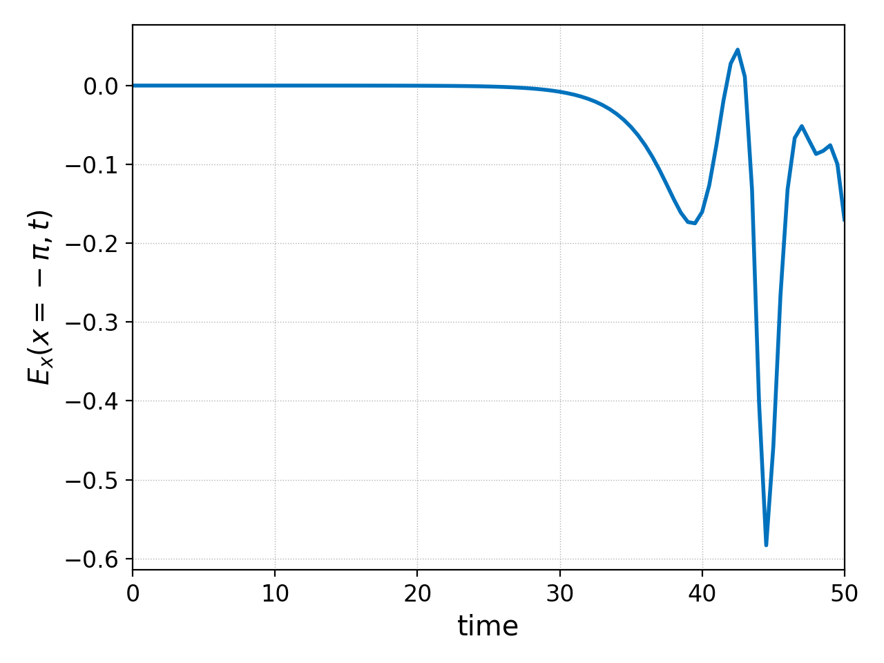
We will sometimes use the abbreviation sel instead of select
for convenience. The resulting figure (above) shows how the amplitude of
the electric field at this point drastically increases as the instability
develops. There is an oscillatory behavior that is lost in this
exponential growth; if one zoomed into the earlier times of this plot,
such oscillations would become visible.
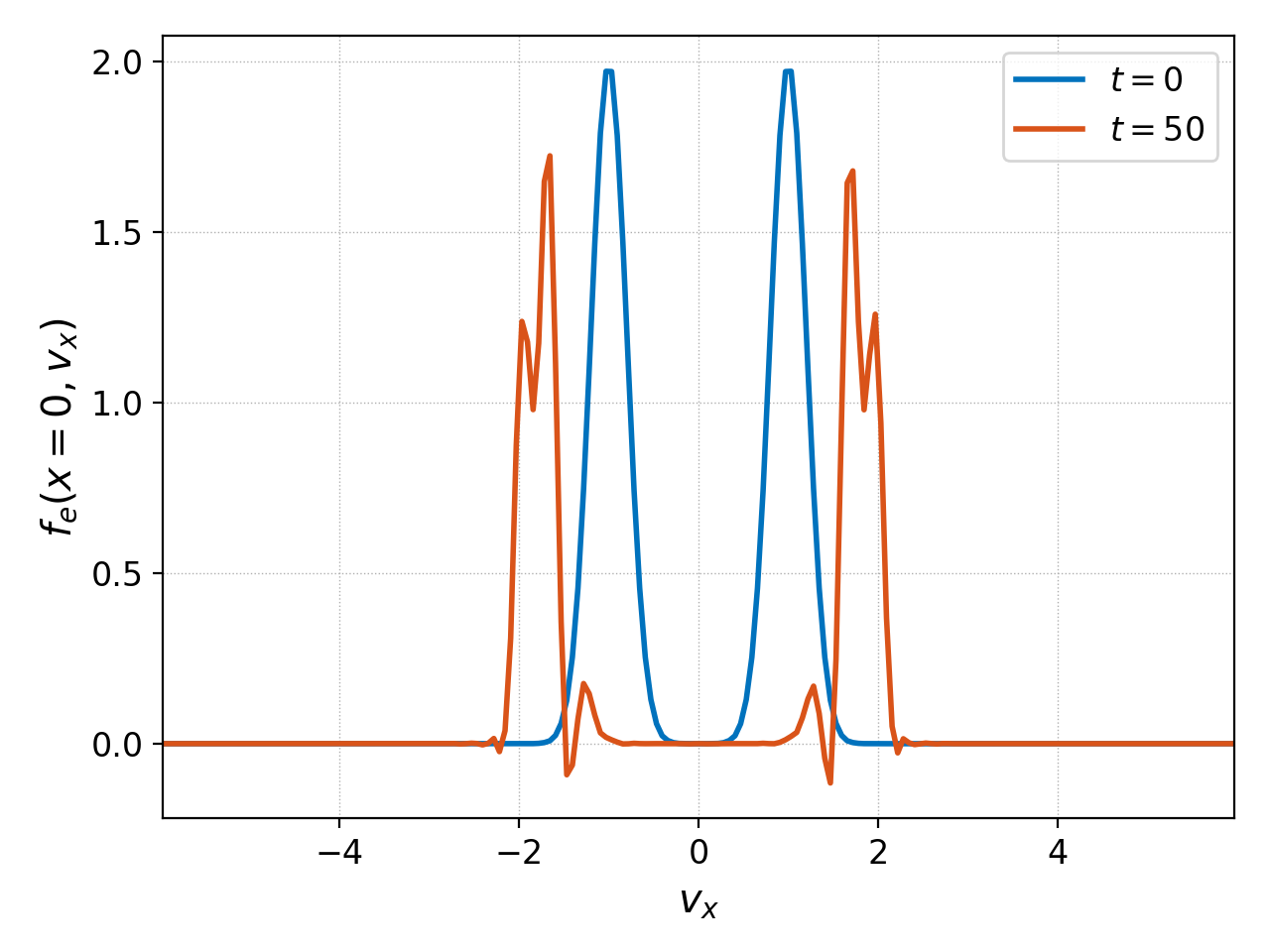
One can, and must, select coordinates at which to evaluate higher (than 2) dimensional datasets. Take the initial and final distribution functions of the electrons as an example; we can evaluate them at \(x=0\) and plot their variation along \(v_x\) with
pgkyl two-stream_elc_0.bp -l '$t=0$' two-stream_elc_100.bp -l '$t=50$' interp \
  sel --z0 0. pl -x '$v_x$' -y '$f_e(x=0,v_x)$' -f0
producing the following plot:
If we were interested in investigating the distribution function in a specific cell along \(x\), say the first (0th in 0-index), we could use
pgkyl two-stream_elc_100.bp sel --z0 0 interp pl -x '$x$' -y '$v_x$'
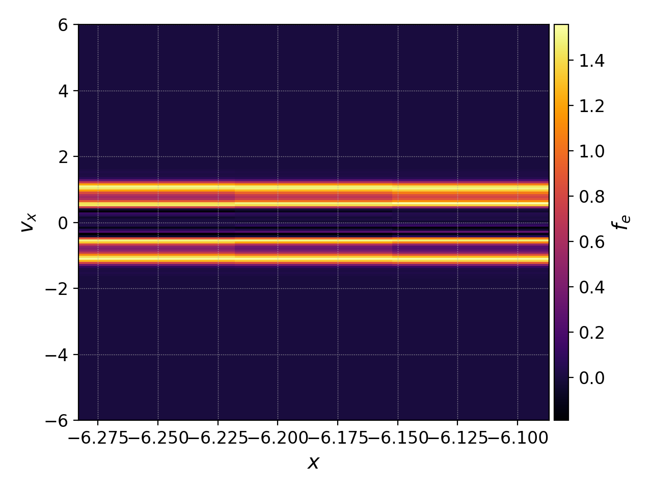
Notice that this produces a 2D colorplot because it takes the expansion coefficients in the 0th cell along \(x\) and all cells along \(v_x\), interpolates them onto a finer mesh and plots them (so the \(x\) extent of this plot is a single cell of the simulation). If we instead wanted a 1D plot of the distribution function along \(v_x\), we could first interpolate onto a finer mesh and then evaluate it at the 0th cell of the finer mesh using
pgkyl two-stream_elc_100.bp interp sel --z0 0 pl -x '$x$' -y '$f_e(x=-6.25046,v_x)$'
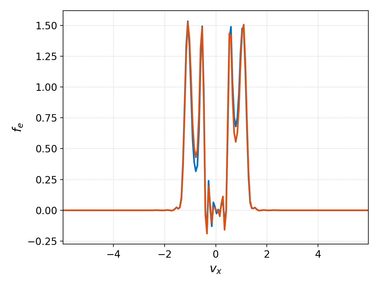
or interpolate it and evaluate it at the lower boundary of the domain along \(x\), which is located at \(x=-2\pi\), with
pgkyl two-stream_elc_100.bp interp sel --z0 -6.283185 pl -x '$x$' -y '$f_e(x=-2\pi,v_x)$'
These two commands are evaluating the distribution function at slightly different \(x\) coordinates (\(\Delta x/(p+1)/2\) apart to be precise, where \(\Delta x\) is the cell length of the simulation, and \(p\) the polynomial order of the basis). We can discern the difference between the two by plotting them together using the following command:
pgkyl two-stream_elc_100.bp -t fe interp sel -t zfl --z0 -6.283185 sel -u fe -t zint --z0 0 \
  pl -u zfl,zint -f0 -x '$v_x$' -y '$f_e$'
This commmand used tags to indicate which dataset to perform the interpolation on, and to name the interpolated datasets. The result is
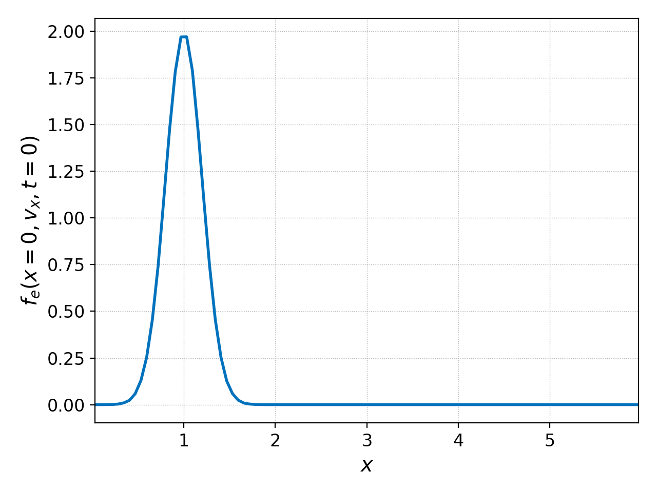
Lastly, we show that the select command can also be used to restrict
and interpolated dataset to a segement along one direction when the
--z# flag is used with a slice of floats. For example, if one wants
to plot the initial electron distribution function at \(x=0\) for
positive velocities only, then one could employ
pgkyl two-stream_elc_0.bp interp sel --z0 0. --z1 0.: pl -x '$x$' -y '$f_e(x=0,v_x,t=0)$'
Script mode
Parameter |
Description |
Default |
|---|---|---|
data (GData) |
Data to subselect. |
|
coord0 (int, float, or slice) |
Index corresponding to the first coordinate for the partial load. Either integer, float, or Python slice (e.g., ‘2:5’). |
None |
coord1 (int, float, or slice) |
Index corresponding to the second coordinate for the partial load. Either integer, float, or Python slice (e.g., ‘2:5’). |
None |
coord2 (int, float, or slice) |
Index corresponding to the third coordinate for the partial load. Either integer, float, or Python slice (e.g., ‘2:5’). |
None |
coord3 (int, float, or slice) |
Index corresponding to the fourth coordinate for the partial load. Either integer, float, or Python slice (e.g., ‘2:5’). |
None |
coord4 (int, float, or slice) |
Index corresponding to the fifth coordinate for the partial load. Either integer, float, or Python slice (e.g., ‘2:5’). |
None |
coord5 (int, float, or slice) |
Index corresponding to the sixth coordinate for the partial load. Either integer, float, or Python slice (e.g., ‘2:5’). |
None |
comp (int, slice, or multiple) |
Index corresponding to the component for the partial load. Either integer, Python slice (e.g., ‘2:5’), or multiple. |
None |
Unlike for the partial load parameters (see :ref:), float point numbers can be specified instead of just integers. In that case, Postgkyl treats it as a grid value and automatically finds and index of a grid point with the closest value. This works both for the single index and for specifying a slice.
In order to use select in a Python script one must interpolate the
nodal/modal dataset in-place (normally it produces a new dataset, i.e. out-of-place)
and pass the original Gkeyll data to the select command. For example, in order to
select the 0-th coordinate at the value 0.0 we would use:
import postgkyl as pg

pgData   = pg.GData(fileName)
pgInterp = pg.GInterpModal(pgData, polyOrder, basisType)
pgInterp.interpolate(overwrite=True)
x, f_z0eq0p0 = pg.data.select(pgData, z0=0.0)
where pg.data.select returns the new grid (x) and the new field (f_z0eq0p0).