Commandline examples¶

There are more examples in the pages describing each of the pgkyl commands and functions. For a brief set of examples we here consider the output of a two-stream instability Vlasov-Maxwell simulation.

List outputs¶

We can list the different kinds of files outputted by the simulation with the listoutputs command

pgkyl list
two-stream_elc
two-stream_elc_M0
two-stream_elc_M1i
two-stream_elc_M2ij
two-stream_elc_M3i
two-stream_field

Notice that we used the abbreviation list instead of listoutputs; this is allowed and whenever convenient we will use abbreviations if the meaning is clear. This writes out a list of the unique filename stems of the files outputted by a simulation.

Obtain file information¶

Now suppose we wish to know more about one file in particular, say the electron initial condition. We can load the data set and probe it with the info command:

pgkyl two-stream_elc_0.bp info
Set  (default#0)
├─ Time: 0.000000e+00
├─ Frame: 0
├─ Number of components: 8
├─ Number of dimensions: 2
├─ Grid: (uniform)
│  ├─ Dim 0: Num. cells: 64; Lower: -6.283185e+00; Upper: 6.283185e+00
│  └─ Dim 1: Num. cells: 64; Lower: -6.000000e+00; Upper: 6.000000e+00
├─ Maximum: 3.804653e+00 at (31, 26) component 0
├─ Minimum: -6.239745e-01 at (31, 38) component 2
├─ DG info:
│  ├─ Polynomial Order: 2
│  └─ Basis Type: serendipity (modal)
├─ Created with Gkeyll:
│  ├─ Changeset: 82231b06678c+
│  └─ Build Date: Feb  7 2021 09:14:06

The output shows (in order):

• Simulation time of this snapshot.

• Frame number of this snapshot.

• Number of degrees of freedom per cell (components). In this case 8 basis functions for the second order 2D Serendipity basis ([Arnold2011], see Modal basis functions for more details).

• Number of dimensions (in this case 2 because it is a 1x1v simulation, 1D in position and 1D in velocity).

• The grid resolution and extents.

• The maximum value of the dataset (in this case largest DG coefficient).

• The minimum value of the dataset (in this case smallest DG coefficient).

• The polynomial order and type of basis.

• The Gkeyll build used to produce this simulation.

Plotting (interpolated data or single coefficients)¶

In the case of DG data one is most frequently interested in plotting the actual function instead of its expansion (DG) coefficients. To do so we construct finite-volume-like dataset on a uniform mesh with higher resolution using the interpolate command. If we interpolate the same dataset (electron initial condition) as in the previous example and inspect it with info, we get

pgkyl two-stream_elc_0.bp interpolate info
Set  (default#0)
├─ Time: 0.000000e+00
├─ Frame: 0
├─ Number of components: 1
├─ Number of dimensions: 2
├─ Grid: (uniform)
│  ├─ Dim 0: Num. cells: 192; Lower: -6.283185e+00; Upper: 6.283185e+00
│  └─ Dim 1: Num. cells: 192; Lower: -6.000000e+00; Upper: 6.000000e+00
├─ Maximum: 1.970512e+00 at (96, 79)
├─ Minimum: -1.177877e-08 at (94, 60)
├─ DG info:
│  ├─ Polynomial Order: 2
│  └─ Basis Type: serendipity (modal)
├─ Created with Gkeyll:
│  ├─ Changeset: 82231b06678c+
│  └─ Build Date: Feb  7 2021 09:14:06

Note that now there is only one degree of freedom (component) per cell but there are 3X more cells; we have interpolated the function onto a finer mesh.

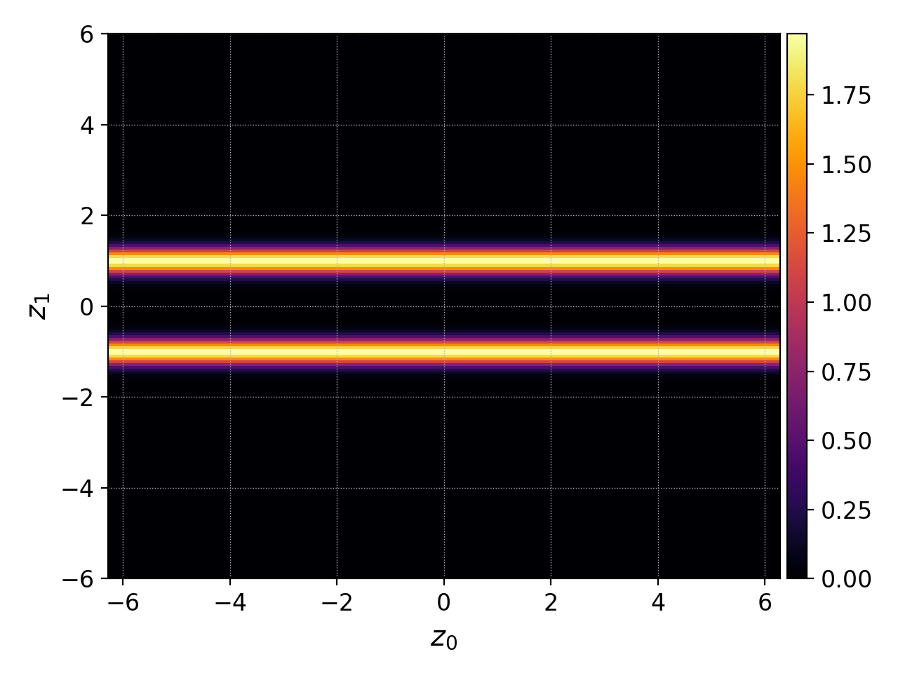
We can then plot the distribution function evaluated on this finer mesh with the plot command

pgkyl two-stream_elc_0.bp interp plot

Note the allowed abbreviation of interpolate to interp. This command produces the figure below:

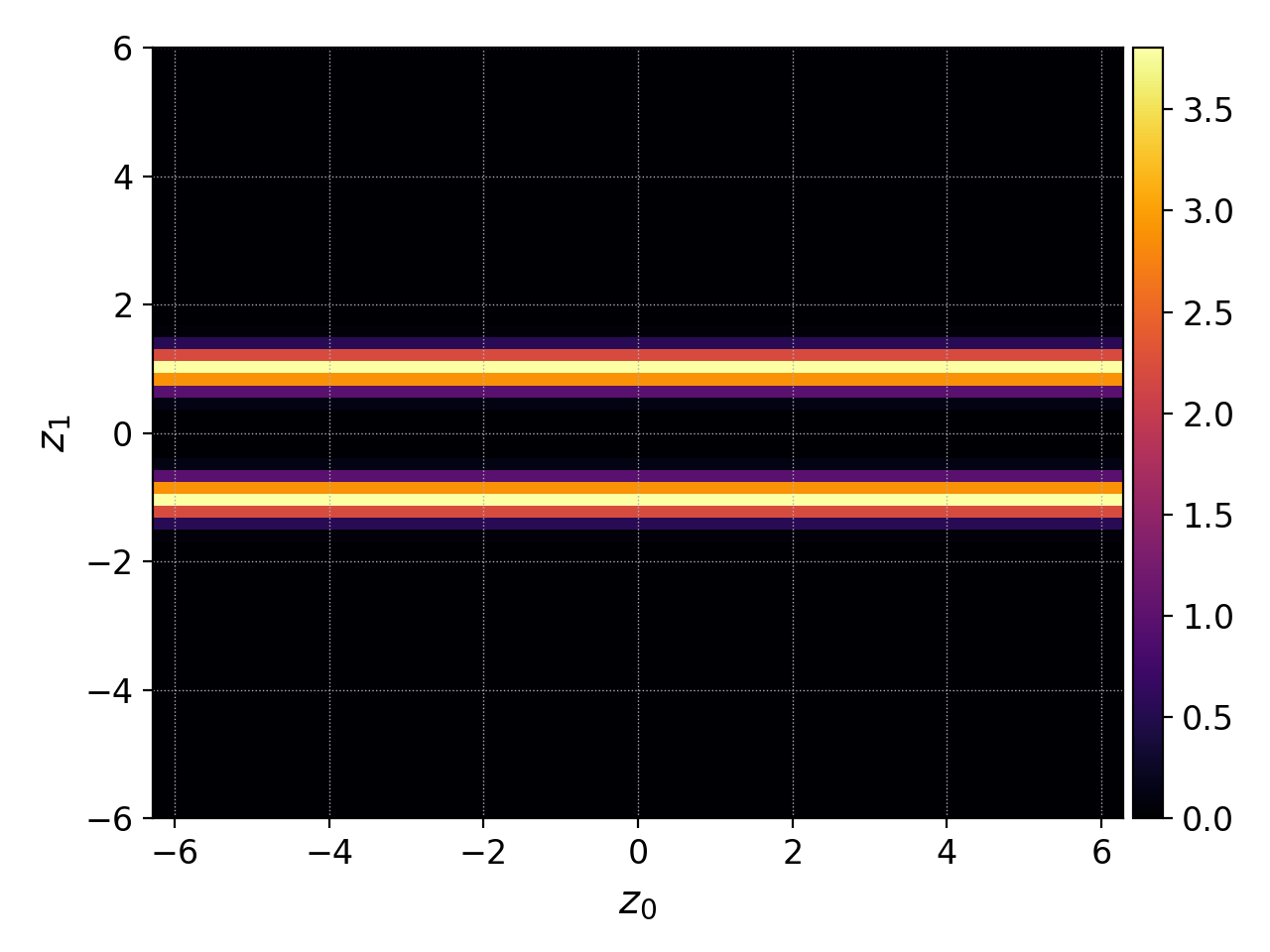
In some cases one may also be interested in plotting single expansion coefficients. The most common use is to, for example, plot the cell-averaged value (which is the zeroth coefficient times a constant). We can select specific coefficients in all cells with the select and the -c flag. So, to plot the cell averaged electron distribution function (times a factor) we would use

pgkyl two-stream_elc_0.bp select -c0 plot

Which produces the figure below. Notice how the values are slightly different and the resolution is coarser than in the previous plot of interpolated data.

Plot data slices¶

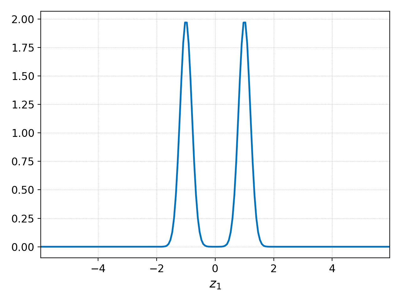
The select command introduced in the previous example can also be used with the --z flag in order to select a data slice which we may subsequently plot. In the two stream instability example, the electron initial condition is clearly independent of position, so we can plot as a function of velocity space at \(x=-2.0\) with

pgkyl two-stream_elc_0.bp interp select --z0 -2. plot

producing the following plot

Postgkyl is currently limited to 1D and 2D plots, so in order to visualize datasets that have more than 3 dimensions one may need to select several slices at once. You can do that with multiple --z flags. For example, if we have a 2x2v simulation producing four-dimensional distribution functions, we can select a slice at \(v_x=0.\) and \(v_y=1.\) with --z2 0. --z3 1..

Create animations¶

Another useful operation is to load multiple datasets consisting of consecutive frames in a time-dependent simulation, plot them and stitch them together into a movie. This can be accomplished by the animate command. We first load all the frames containing the electron momentum densities in time (i.e. elc_M1i), then interpolate them onto a finer mesh, and put together all the frames with the animate command:

pgkyl "two-stream_elc_M1i_[0-9]*.bp" interp animate -x 'x' -y 'Momentum'

Here we are also using the -x and -y flags to the animate command in order to place labels in the figure. The product is the movie given below:

Of course, one can use command chaining to slice higher dimensional data prior to calling the animate command. For example, creating an animation of the distribution function along velocity-space at \(x=0\) would be accomplished with

pgkyl "two-stream_elc_[0-9]*.bp" interp sel --z0 0. animate

Here we have used the abbreviations interp and sel in favor of interpolate and select, respectively. Such command produces this animation:

Averaging and integrating¶

A common diagnostic need is to perform averages and integrations over a dimension or over time. In general averages can be performed either by using the ev command with the avg operation, or using the integrate and later dividing by the corresponding space/time segment (with the ev command).

We use the final electron distribution function (frame 100) as an example. Let’s first plot it in phase-space to get a sense of it:

pgkyl two-stream_elc_100.bp interp pl

Suppose we wish to average over the central region \(x\in[-2,2]\) where a velocity-space ‘hole’ forms. We can plot such \(x\) integral as follows

pgkyl two-stream_elc_100.bp interp sel --z0 -2.:2. ev 'f[0] 0 avg' pl

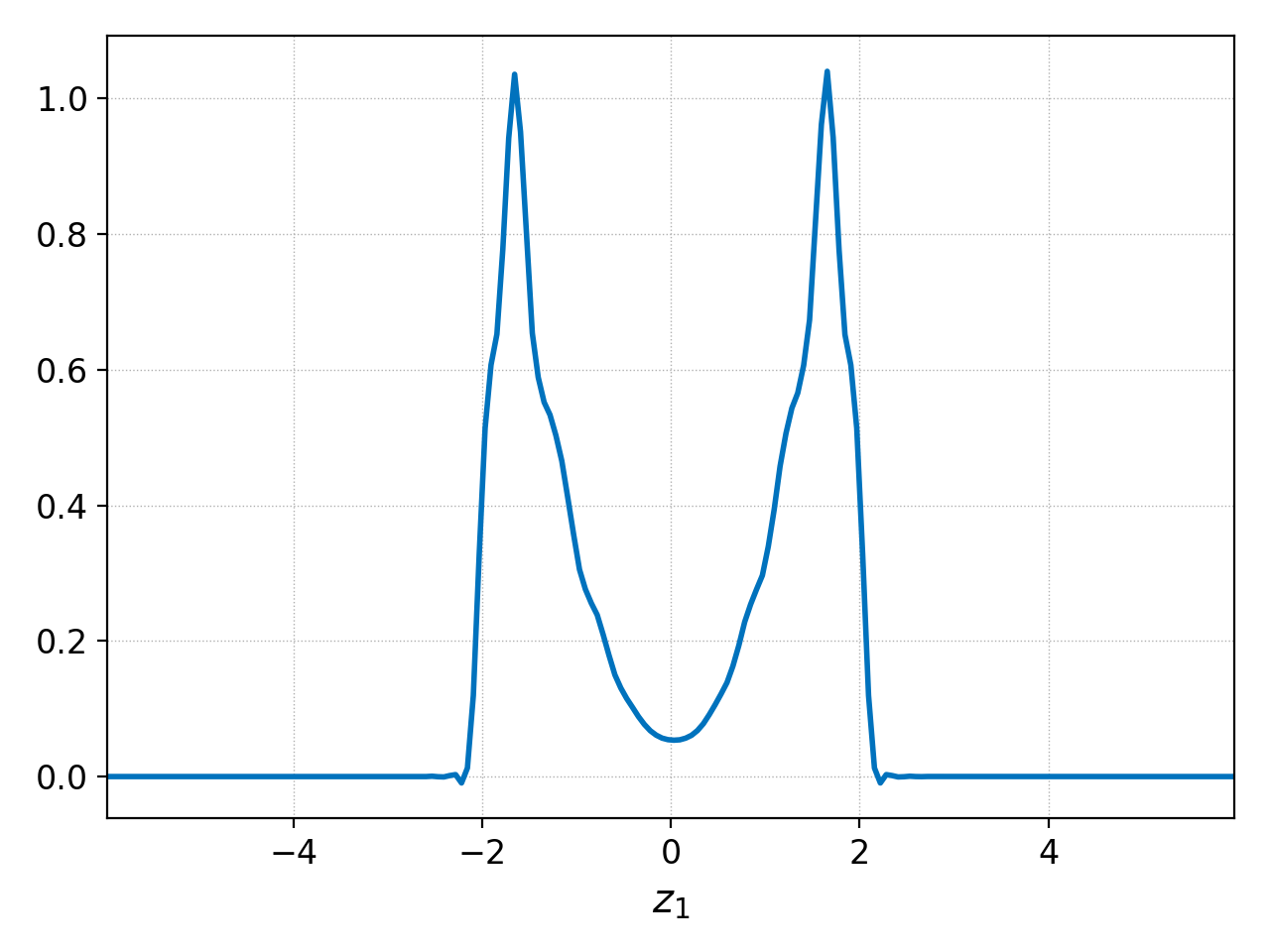
As mentioned above, we can also do this with the integrate command. We accomplish that with

pgkyl two-stream_elc_100.bp interp sel --z0 -2.:2. integrate 0 ev 'f[0] 4. /' pl

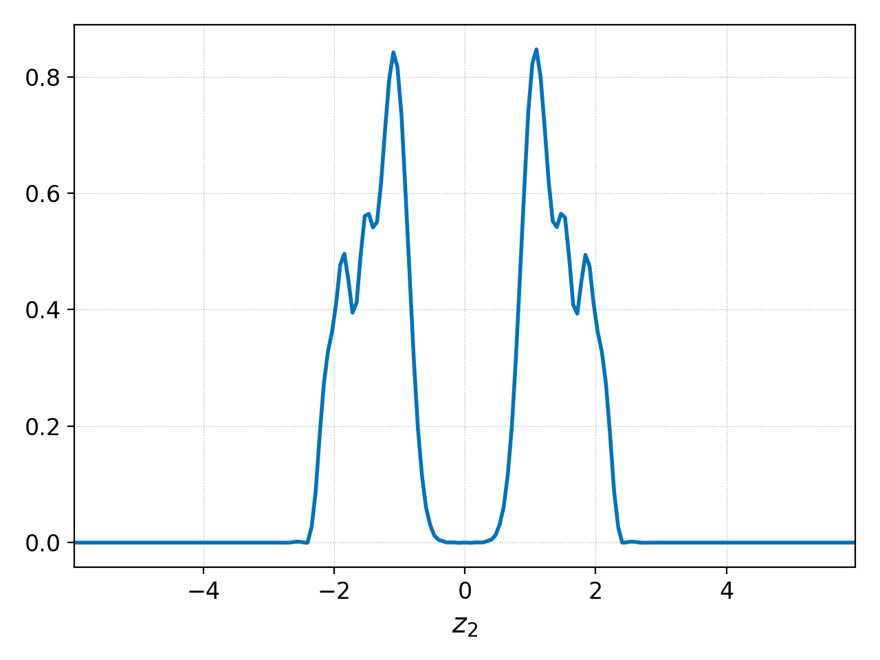
Another useful application of ev (with avg) and integrate is to average or integrate quantities over time. Consider the evolution of the electron distribution function along velocity space at \(x=0\) in the previous example. The action starts after the 60th frame approximately, so if we wish to time-average the distribution function at \(x=0\) we could use the ev command as follows:

pgkyl "two-stream_elc_[0-9]*.bp" activate -i '59:' interp sel --z0 0. collect ev 'f[0] 0 avg' pl

A different way to accomplish the same time average over frames 59-100 and dividing by the corresponding time period (\(\tau=50-29.5018=20.4982\)):

pgkyl "two-stream_elc_[0-9]*.bp" activate -i '59:' interp sel --z0 0. collect integrate 0 ev 'f[0] 20.4982 /' pl

To break this last approach down, the command does the following (in order):

• Load all frames of the electron distribution function.

• Activate only frames 59-100.

• Interpolate each frame onto a finer mesh and slice at \(x=0\).

• Collect all the slices into a single dataset. This produces a 2D dataset with time along the 0th dimension and velocity-space along the 1st dimension.

• Use the integrate command to integrate along the 0th dimension (time).

• Use ev to divide the time-integrated quantity by the appropriate time window.

• Plot.

The product of either of these comands is shown below:

Plot differences between datasets¶

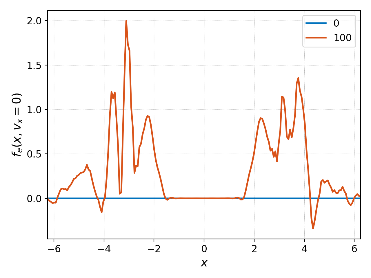
It is common to have to evaluate the difference between two datasets. These could be two frames from the same simulation, or two datasets from different simulations. There are also various ways to discern differences, and below we show how to plot them in a single figure or how to plot their actual difference.

Suppose we wish to see how the electron distribution function has changed along \(x\) between \(t=0\) (0th frame) and \(t=50\) (100th frame) at \(v_x=0\). We can plot both of these datasets as follows

pgkyl two-stream_elc_0.bp two-stream_elc_100.bp interp sel --z1 0. plot -f0 -x '$x$' -y '$f_e(x,v_x=0)$'

where we have specified the figure with -f0 so they are both plotted together, and we have used -x and -y to place labels. The plot produced is

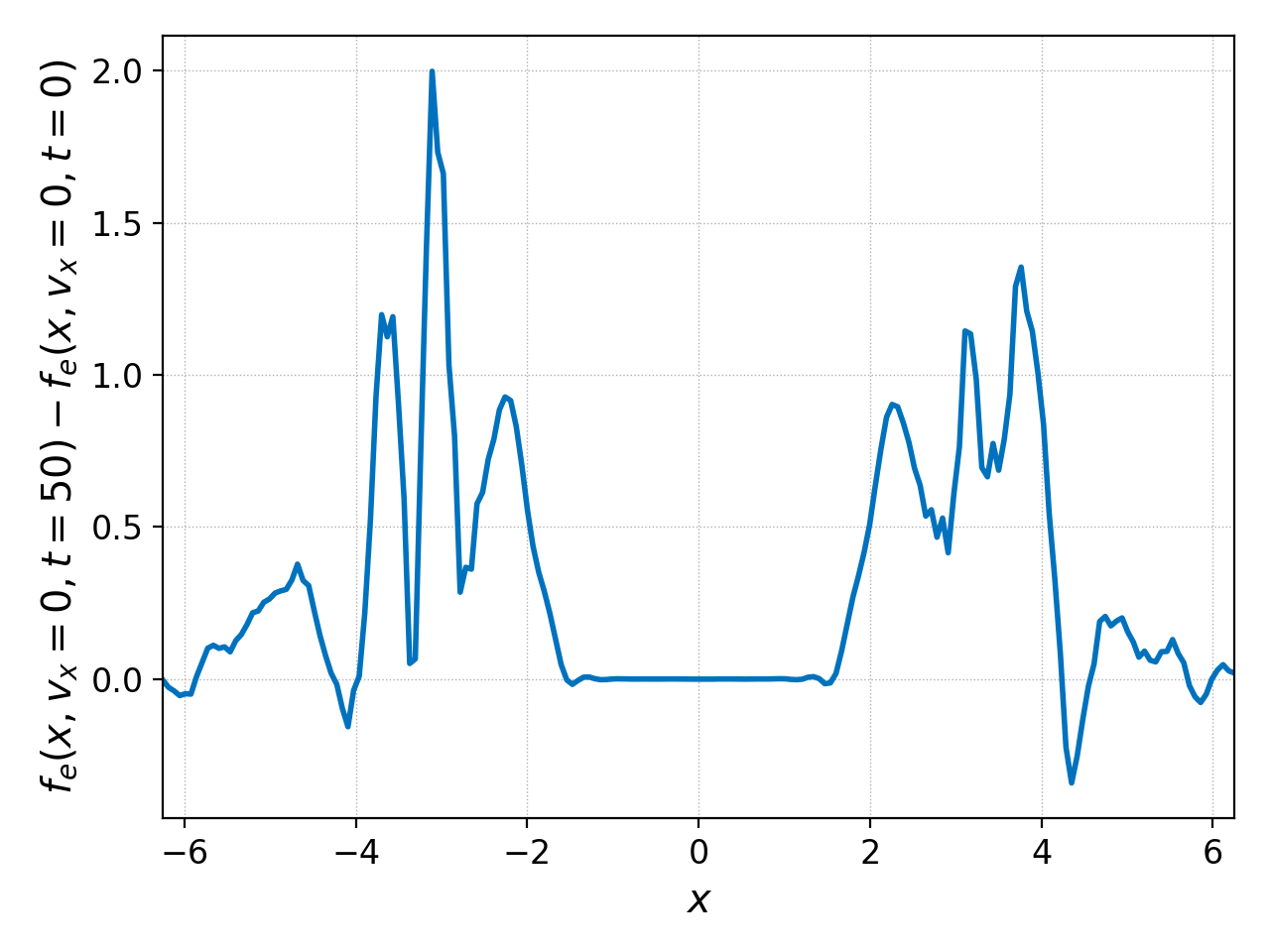
Another alternative is to compute the actual difference of the two data sets with ev:

pgkyl two-stream_elc_0.bp two-stream_elc_100.bp interp sel --z1 0. ev 'f[1] f[0] -' pl

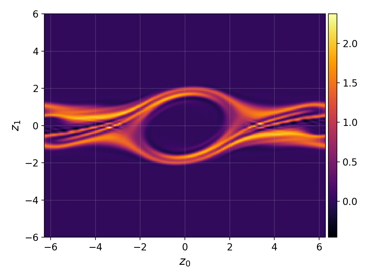
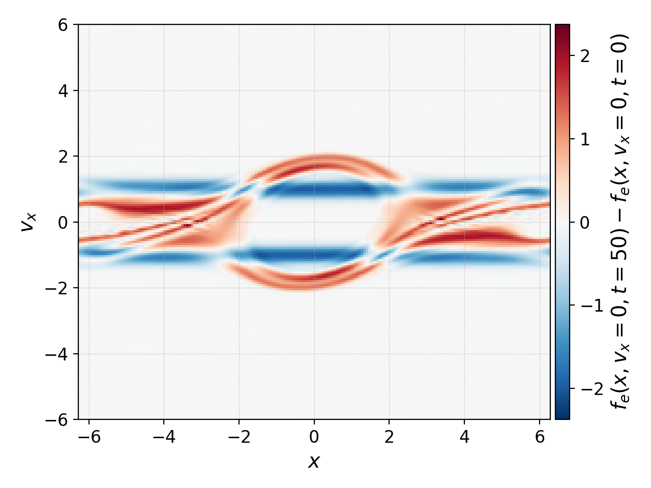
Note that these operations also work with 2D datasets. So we could’ve have taken the whole distribution function in phase space at \(t=0,50\), subtracted them and plot them with

pgkyl two-stream_elc_0.bp two-stream_elc_100.bp interp ev 'f[1] f[0] -' plot --diverging

which thanks to the --diverging flag, produces the following image:

Saving plots/animations to a file¶

Any of the figures above can be saved to a file by appending either --save, or --saveas followed by the desired filename. For example the diverging 2D colorplot in the previous section can be saved to a file with

pgkyl two-stream_elc_0.bp two-stream_elc_100.bp interp ev 'f[1] f[0] -' plot --diverging --saveas 'two-stream_elc_fr0m100.png'

Fileformats supported depend on matplotlib, but likely include .png, .pdf and .eps.

The animate command is also capable of saving animations to a file. It requires an ffmpeg installation, and once that is available we can create an animation described earlier as

pgkyl "two-stream_elc_[0-9]*.bp" interp sel --z0 0. animate --saveas 'two-stream_elc_z0eq0p0.mp4'

Extracting input file¶

In our commitment to reproducibility, Gkeyll output files store the Lua input file used to produce that data. This input file can be extracted using the extractinput command, as follows

pgkyl two-stream_elc_0.bp extractinput

By default, this commands simply prints the input file to screen. However, this could be easily piped into a new file with

pgkyl two-stream_elc_0.bp extractinput > newInputFile.lua

Reference¶