Gyrokinetic example
The gyrokinetic system is used to study turbulence in magnetized plasmas. Gkeyll’s Gyrokinetic App is specialized to study the edge/scrape-off-layer region of fusion devices, which requires handling of large fluctuations and open-field-line regions. In this example, we will set up a gyrokinetic problem on open magnetic field lines (e.g. in the tokamak scrape-off layer). Using specialized boundary conditions along the field line that model the sheath interaction between the plasma and conducting end plates, we will see that we can model the self-consistent formation of the sheath potential. This simple test case can then be used as a starting point for full nonlinear simulations of the tokamak SOL.
Input file
The full Lua input file (gk-sheath.lua) for this simulation is a bit longer than the one in A first Gkeyll simulation, but not to worry, we will go through each part of the input file carefully.
To set up a gyrokinetic simulation, we first need to load the
Gyrokinetic App package and other dependencies. This should be done
at the top of the input file, via
--------------------------------------------------------------------------------
-- App dependencies
--------------------------------------------------------------------------------
local Plasma    = require("App.PlasmaOnCartGrid").Gyrokinetic()   -- load the Gyrokinetic App
local Constants = require "Lib.Constants"                         -- load some physical Constants
Here we have also loaded the Constants library, which
contains various physical constants that we will use later.
The next block is the Preamble, containing input paramters and simple derived quantities:
--------------------------------------------------------------------------------
-- Preamble
--------------------------------------------------------------------------------
-- Universal constant parameters.
eps0 = Constants.EPSILON0
eV = Constants.ELEMENTARY_CHARGE
qe = -eV                             -- electron charge
qi = eV                              -- ion charge
me = Constants.ELECTRON_MASS         -- electron mass
mi = 2.014*Constants.PROTON_MASS     -- ion mass (deuterium ions)

-- Plasma parameters.
Te0 = 40*eV                          -- reference electron temperature, used to set up electron velocity grid [eV]
Ti0 = 40*eV                          -- reference ion temperature, used to set up ion velocity grid [eV]
n0 = 7e18                            -- reference density [1/m^3]

-- Geometry and magnetic field parameters.
B_axis = 0.5                         -- magnetic field strength at magnetic axis [T]
R0 = 0.85                            -- device major radius [m]
a0 = 0.15                            -- device minor radius [m]
R = R0 + a0                          -- major radius of flux tube simulation domain [m]
B0 = B_axis*(R0/R)                   -- magnetic field strength at R [T]
Lpol = 2.4                           -- device poloidal length (e.g. from bottom divertor plate to top) [m]

-- Parameters for collisions.
nuFrac = 0.1                         -- use a reduced collision frequency (10% of physical)
-- Electron collision freq.
logLambdaElc = 6.6 - 0.5*math.log(n0/1e20) + 1.5*math.log(Te0/eV)
nuElc = nuFrac*logLambdaElc*eV^4*n0/(6*math.sqrt(2)*math.pi^(3/2)*eps0^2*math.sqrt(me)*(Te0)^(3/2))
-- Ion collision freq.
logLambdaIon = 6.6 - 0.5*math.log(n0/1e20) + 1.5*math.log(Ti0/eV)
nuIon = nuFrac*logLambdaIon*eV^4*n0/(12*math.pi^(3/2)*eps0^2*math.sqrt(mi)*(Ti0)^(3/2))

-- Derived parameters
vti = math.sqrt(Ti0/mi)              -- ion thermal speed
vte = math.sqrt(Te0/me)              -- electron thermal speed
c_s = math.sqrt(Te0/mi)              -- ion sound speed
omega_ci = math.abs(qi*B0/mi)        -- ion gyrofrequency
rho_s = c_s/omega_ci                 -- ion sound gyroradius

-- Simulation box size
Lx = 50*rho_s                        -- x = radial direction
Ly = 100*rho_s                       -- y = binormal direction
Lz = 4                               -- z = field-aligned direction
This simulation also requires a source, which models plasma crossing the separatrix. The next part of the Preamble initializes some source parameters, along with some functions that will be used later to set up the source density and temperature profiles.
-- Source parameters
P_SOL = 3.4e6                          -- total SOL power, from experimental heating power [W]
P_src = P_SOL*Ly*Lz/(2*math.pi*R*Lpol) -- fraction of total SOL power into flux tube domain [W]
xSource = R                            -- source peak radial location [m]
lambdaSource = 0.005                   -- source radial width [m]

-- Source density and temperature profiles.
-- Note that source density will be scaled to achieve desired source power.
sourceDensity = function (t, xn)
   local x, y, z = xn[1], xn[2], xn[3]
   local sourceFloor = 1e-10
   if math.abs(z) < Lz/4 then
      -- near the midplane, the density source is a Gaussian
      return math.max(math.exp(-(x-xSource)^2/(2*lambdaSource)^2), sourceFloor)
   else
      return 1e-40
   end
end
sourceTemperature = function (t, xn)
   local x, y, z = xn[1], xn[2], xn[3]
   if math.abs(x-xSource) < 3*lambdaSource then
      return 80*eV
   else
      return 30*eV
   end
end
This concludes the Preamble. We now have everything we need to initialize
the Gyrokinetic App. In this input file, the App initialization consists
of 4 sections:
--------------------------------------------------------------------------------
-- App initialization
--------------------------------------------------------------------------------
plasmaApp = Plasma.App {
   -----------------------------------------------------------------------------
   -- Common
   -----------------------------------------------------------------------------
   ...

   -----------------------------------------------------------------------------
   -- Species
   -----------------------------------------------------------------------------
   ...

   -----------------------------------------------------------------------------
   -- Fields
   -----------------------------------------------------------------------------
   ...

   -----------------------------------------------------------------------------
   -- Geometry
   -----------------------------------------------------------------------------
   ...
}
The Common section includes a declaration of parameters that control the
(configuration space) discretization, and time advancement. This first block of
code in Plasma.App may specify the periodic directions, the MPI
decomposition, and the frequency with which to output certain diagnostics.
-----------------------------------------------------------------------------
-- Common
-----------------------------------------------------------------------------
logToFile = true,                    -- will write simulation output log to gk-sheath_0.log
tEnd = 10e-6,                        -- simulation end time [s]
nFrame = 10,                          -- number of output frames for diagnostics
lower = {R - Lx/2, -Ly/2, -Lz/2},    -- configuration space domain lower bounds, {x_min, y_min, z_min}
upper = {R + Lx/2, Ly/2, Lz/2},      -- configuration space domain upper bounds, {x_max, y_max, z_max}
cells = {4, 1, 8},                   -- number of configuration space cells, {nx, ny, nz}
basis = "serendipity",               -- basis type (only "serendipity" is supported for gyrokinetics)
polyOrder = 1,                       -- polynomial order of basis set (polyOrder = 1 fully supported for gyrokinetics, polyOrder = 2 marginally supported)
timeStepper = "rk3",                 -- timestepping algorithm
cflFrac = 0.8,                       -- fractional modifier for timestep calculation via CFL condition
restartFrameEvery = .2,              -- restart files will be written after every 20% of simulation

-- Specification of periodic directions
-- (1-based indexing, so x-periodic = 1, y-periodic = 2, etc)
periodicDirs = {2},     -- Periodic in y only (y = 2nd dimension)
The Species section sets up the species to be considered in the simulation.
Each species gets its own Lua table, in which one provides the velocity-space domain and discretization of the species, initial conditions, sources, collisions, boundary conditions, and diagnostics.
In this input file, we initialize gyrokinetic electron and ion species. Since this section is the most involved part of the input file, we will discuss various parts in detail below.
--------------------------------------------------------------------------------
-- Species
--------------------------------------------------------------------------------
-- Gyrokinetic electrons
electron = Plasma.Species {
   evolve = true,     -- evolve species?
   charge = qe,       -- species charge
   mass = me,         -- species mass

   -- Species-specific velocity domain
   lower = {-4*vte, 0},                    -- velocity space domain lower bounds, {vpar_min, mu_min}
   upper = {4*vte, 12*me*vte^2/(2*B0)},    -- velocity space domain upper bounds, {vpar_max, mu_max}
   cells = {8, 4},                         -- number of velocity space cells, {nvpar, nmu}

   -- Initial conditions
   init = Plasma.MaxwellianProjection {    -- initialize a Maxwellian with the specified density and temperature profiles
      -- density profile
      density = function (t, xn)
         -- The particular functional form of the initial density profile
         -- comes from a 1D single-fluid analysis (see Shi thesis), which derives
         -- quasi-steady-state initial profiles from the source parameters.
         local x, y, z, vpar, mu = xn[1], xn[2], xn[3], xn[4], xn[5]
         local Ls = Lz/4
         local floor = 0.1
         local effectiveSource = math.max(sourceDensity(t,{x,y,0}), floor)
         local c_ss = math.sqrt(5/3*sourceTemperature(t,{x,y,0})/mi)
         local nPeak = 4*math.sqrt(5)/3/c_ss*Ls*effectiveSource/2
         local perturb = 0
         if math.abs(z) <= Ls then
            return nPeak*(1+math.sqrt(1-(z/Ls)^2))/2*(1+perturb)
         else
            return nPeak/2*(1+perturb)
         end
      end,
      -- temperature profile
      temperature = function (t, xn)
         local x = xn[1]
         if math.abs(x-xSource) < 3*lambdaSource then
            return 50*eV
         else
            return 20*eV
         end
      end,
      scaleWithSourcePower = true,     -- when source is scaled to achieve desired power, scale initial density by same factor
   },

   -- Collisions parameters
   coll = Plasma.LBOCollisions {          -- Lenard-Bernstein model collision operator
      collideWith = {'electron'},         -- only include self-collisions with electrons
      frequencies = {nuElc},              -- use a constant (in space and time) collision freq. (calculated in Preamble)
   },

   -- Source parameters
   source = Plasma.Source {              -- source is a Maxwellian with the specified density and temperature profiles
      density = sourceDensity,           -- use sourceDensity function (defined in Preamble) for density profile
      temperature = sourceTemperature,   -- use sourceTemperature function (defined in Preamble) for temperature profile
      power = P_src/2,                   -- sourceDensity will be scaled to achieve desired power
      diagnostics = {"intKE"},
   },

   polarizationDensityFactor = n0,  -- Density used in polarization density.

   -- Non-periodic boundary condition specification
   bcx = {Plasma.ZeroFluxBC{diagnostics={"M0", "Energy", "intM0", "intM1", "intKE", "intEnergy"}},
          Plasma.ZeroFluxBC{diagnostics={"M0", "Energy", "intM0", "intM1", "intKE", "intEnergy"}}},   -- use zero-flux boundary condition in x direction
   bcz = {Plasma.SheathBC{diagnostics={"M0", "Energy", "intM0", "intM1", "intKE", "intEnergy"}},
          Plasma.SheathBC{diagnostics={"M0", "Energy", "intM0", "intM1", "intKE", "intEnergy"}}},       -- use sheath-model boundary condition in z direction

   -- Diagnostics
   diagnostics = {"M0", "Upar", "Temp", "intM0", "intM1", "intKE", "intEnergy"},
},

-- Gyrokinetic ions
ion = Plasma.Species {
   evolve = true,     -- evolve species?
   charge = qi,       -- species charge
   mass = mi,         -- species mass

   -- Species-specific velocity domain
   lower = {-4*vti, 0},                    -- velocity space domain lower bounds, {vpar_min, mu_min}
   upper = {4*vti, 12*mi*vti^2/(2*B0)},    -- velocity space domain upper bounds, {vpar_max, mu_max}
   cells = {8, 4},                         -- number of velocity space cells, {nvpar, nmu}

   -- Initial conditions
   init = Plasma.MaxwellianProjection {    -- initialize a Maxwellian with the specified density and temperature profiles
      -- density profile
      density = function (t, xn)
         -- The particular functional form of the initial density profile
         -- comes from a 1D single-fluid analysis (see Shi thesis), which derives
         -- quasi-steady-state initial profiles from the source parameters.
         local x, y, z, vpar, mu = xn[1], xn[2], xn[3], xn[4], xn[5]
         local Ls = Lz/4
         local floor = 0.1
         local effectiveSource = math.max(sourceDensity(t,{x,y,0}), floor)
         local c_ss = math.sqrt(5/3*sourceTemperature(t,{x,y,0})/mi)
         local nPeak = 4*math.sqrt(5)/3/c_ss*Ls*effectiveSource/2
         local perturb = 0
         if math.abs(z) <= Ls then
            return nPeak*(1+math.sqrt(1-(z/Ls)^2))/2*(1+perturb)
         else
            return nPeak/2*(1+perturb)
         end
      end,
      -- temperature profile
      temperature = function (t, xn)
         local x = xn[1]
         if math.abs(x-xSource) < 3*lambdaSource then
            return 50*eV
         else
            return 20*eV
         end
      end,
      scaleWithSourcePower = true,     -- when source is scaled to achieve desired power, scale initial density by same factor
   },

   -- Collisions parameters
   coll = Plasma.LBOCollisions {     -- Lenard-Bernstein model collision operator
      collideWith = {'ion'},         -- only include self-collisions with ions
      frequencies = {nuIon},         -- use a constant (in space and time) collision freq. (calculated in Preamble)
   },

   -- Source parameters
   source = Plasma.Source {       -- source is a Maxwellian with the specified density and temperature profiles
      density = sourceDensity,           -- use sourceDensity function (defined in Preamble) for density profile
      temperature = sourceTemperature,   -- use sourceTemperature function (defined in Preamble) for temperature profile
      power = P_src/2,                   -- sourceDensity will be scaled to achieve desired power
      diagnostics = {"intKE"},
   },

   polarizationDensityFactor = n0,  -- Density used in polarization density.

   -- Non-periodic boundary condition specification
   bcx = {Plasma.ZeroFluxBC{diagnostics={"M0", "Energy", "intM0", "intM1", "intKE", "intEnergy"}},
          Plasma.ZeroFluxBC{diagnostics={"M0", "Energy", "intM0", "intM1", "intKE", "intEnergy"}}},   -- use zero-flux boundary condition in x direction
   bcz = {Plasma.SheathBC{diagnostics={"M0", "Energy", "intM0", "intM1", "intKE", "intEnergy"}},
          Plasma.SheathBC{diagnostics={"M0", "Energy", "intM0", "intM1", "intKE", "intEnergy"}}},       -- use sheath-model boundary condition in z direction

   -- Diagnostics
   diagnostics = {"M0", "Upar", "Temp", "intM0", "intM1", "intKE", "intEnergy"},
},
The initial condition for this problem is given by a Maxwellian. This
is specified using init = Plasma.MaxwellianProjection { ... },
which is a table with entries for the density and temperature profile
functions (we could also specify the driftSpeed profile) to be used
to initialze the Maxwellian. In this simulation, the initial density
profile takes a particular form that comes from a 1D single-fluid
analysis (see [Shi2019]), which derives quasi-steady-state initial
profiles from the source parameters.
By default the sources, specified via
source = Plasma.Source { ... }, also take the form of Maxwellians.
For the density and temperature profile functions, we use the
sourceDensity and sourceTemperature functions defined in the
Preamble. We also specify the desired source power. The source density
is then scaled so that the integrated power in the source matches the
desired power. Therefore, sourceDensity only controls the shape of the
source density profile, not the amplitude. Since the initial conditions
are related to the source, we also scale the initial species density
by the same factor as the source via the scaleWithSourcePower = true
flag in the initial conditions.
Self-species collisions are included using a Lenard-Bernstein model
collision operator via the coll = Plasma.LBOCollisions { ... } table.
For more details about collision models and options, see
Collisions.
Non-periodic boundary conditions are specified via the bcx and bcz
tables. For this simulation, we use zero-flux boundary conditions in the
\(x\) (radial) direction, and sheath-model boundary conditions in the
\(z\) (field-aligned) direction.
Finally, we specify the diagnostics that should be outputted for each species. These consist of various moments and integrated quantities. For more details about available diagnostics, see Gyrokinetic App: Electromagnetic gyrokinetic model for magnetized plasmas.
The Fields section specifies parameters and options related to the
field solvers for the gyrokinetic potential(s).
--------------------------------------------------------------------------------
-- Fields
--------------------------------------------------------------------------------
-- Gyrokinetic field(s)
field = Plasma.Field {
   evolve = true, -- Evolve fields?
   isElectromagnetic = false,  -- use electromagnetic GK by including magnetic vector potential A_parallel?

   -- Boundary condition specification for electrostatic potential phi.
   -- Dirichlet in x. Periodic in y. No BC required in z (Poisson solve is only in
   -- perpendicular x,y directions)
   bcLowerPhi  = {{T = "D", V = 0.0}, {T = "P"}},
   bcUpperPhi  = {{T = "D", V = 0.0}, {T = "P"}},
},
The Geometry section specifies parameters related to the
background magnetic field and other geometry parameters.
--------------------------------------------------------------------------------
-- Geometry
--------------------------------------------------------------------------------
-- Magnetic geometry
externalField = Plasma.Geometry {
   -- Background magnetic field profile
   -- Simple helical (i.e. cylindrical slab) geometry is assumed
   bmag = function (t, xn)
      local x = xn[1]
      return B0*R/x
   end,
quantity is controlled by the nFrame parameter in the input file.
Finally, an input file concludes with an invocation of the App’s run method:
--------------------------------------------------------------------------------
-- Run the App
--------------------------------------------------------------------------------
plasmaApp:run()
We can use the Gkeyll post-processing tool (postgkyl) to visualize the outputs.
Electron density and distribution function
First, let’s examine the initial conditions, which are given in output file
sending in _0.bp. The initial electron density \(n_e(x,y,z)\) is
found in gk-sheath_electron_M0_0.bp, where M0 is the label for
the density moment. Let’s look at this file as a function of the \(x\)
and \(z\) coordintes by taking a line-out at \(y=0\) via
pgkyl gk-sheath_electron_M0_0.bp interp sel --z1 0. pl -x '$x$' -y '$z$'
where we have used the interp (interpolate)
command to interpolate the DG data onto the grid, and the sel --z1 0.
(select) command to make the line-out at \(y=0\)
(--z1 refers to the \(y\) coordinate here). The resulting plot looks like
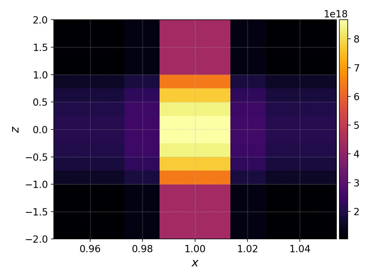
Initial electron density \(n_e(x,y=0,z,t=0)\)
We ran this simulation for 10 \(\mu\text{s}\), and since nframe=10
we have an output frame for each \(\mu\text{s}\) of the simulation.
Let’s look at the final state now, at \(t=10\mu\text{s}\).
pgkyl gk-sheath_electron_M0_10.bp interp sel --z1 0. pl -x '$x$' -y '$z$'
gives
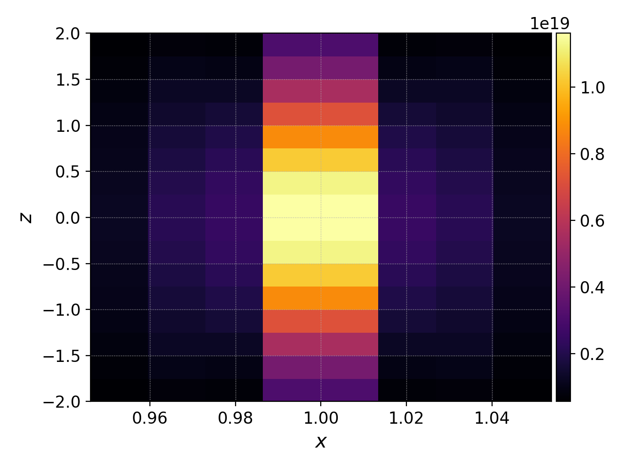
Electron density \(n_e(x,y=0,z,t=10\mu\text{s})\)
Seeing as we have run a kinetic calculation, we may wish to examine the velocity-space structure of the distribution function. From postgkyl’s point of view distribution functions are just another dataset, albeit a higher dimensional one. Since we can only produce 1D and 2D plots at the moment we have to select at least 3 of the 5 coordinates at specific values. We will make a 2D plot of velocity-space at t=0 by selecting (x,y,z)=(1.,0,0), which is near the center of the domain, with the following command:
pgkyl gk-sheath_electron_0.bp interp sel --z0 1. --z1 0. --z2 0. pl -x '$v_\parallel$' -y '$\mu$' --clabel '$f_e(x=1,y=0,z=0,v_\parallel,\mu,t=0)$'
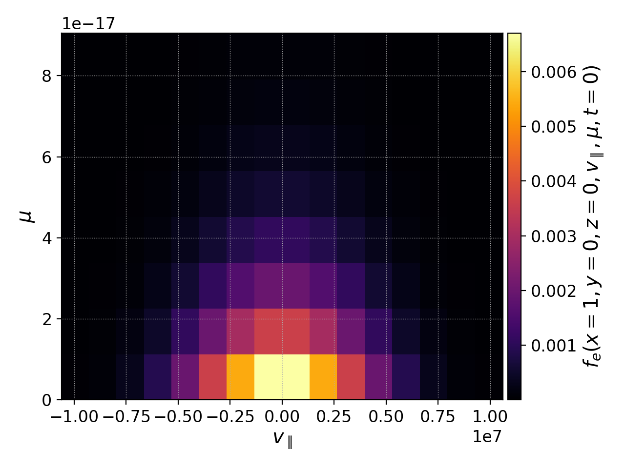
This plot shows that the initial \(f_e\) is Maxwellian. In this example the distribution remains essentially Maxwellian throughout time, so if we were to plot the last frame we would obtain a similar picture.
Sheath potential
Now let’s look at the electrostatic potential, \(\phi\). We’d like to see if the sheath potential formed self-consistently due to our conducting-sheath boundary conditions. Let’s look at \(\phi\) along the field line (i.e. along the \(z\) coordinate) by taking line-outs at \(x=1.0\) and \(y=0\).
pgkyl gk-sheath_phi_10.bp interp sel --z0 1. --z1 0. pl -x '$z$'
gives
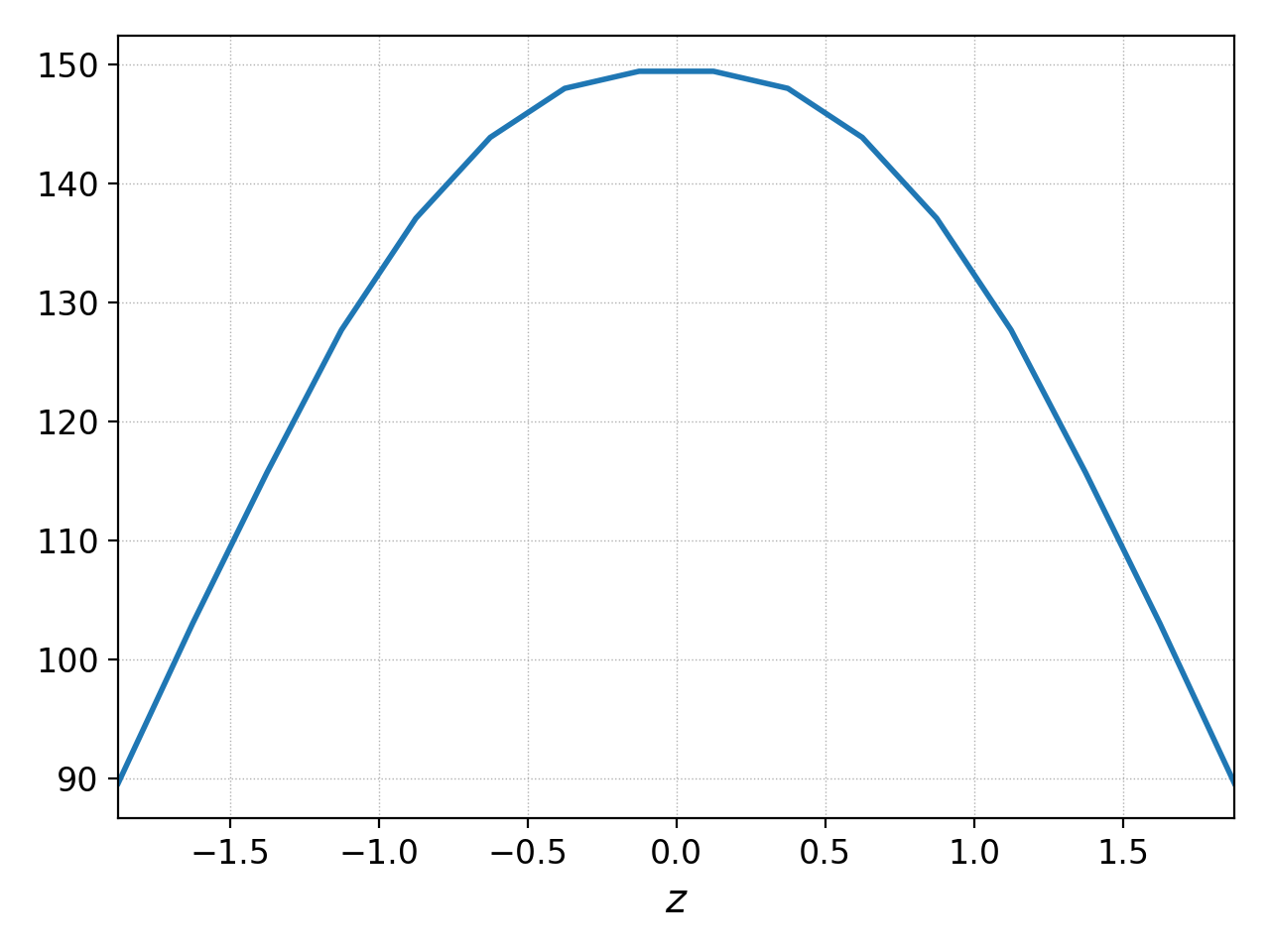
Electrostatic potential \(\phi(x=1,y=0,z,t=10\mu\text{s})\)
Indeed, at the domain ends in \(z\), we have a sheath potential \(\phi_{sh} = 90 \text{ V}\).
We can also make an animation of the evolution of the sheath potential via
pgkyl "gk-sheath_phi_[0-9]*.bp" interp sel --z0 1. --z1 0. anim -x '$z$'
Divertor Fluxes
pgkyl gk-sheath_ion_bcZlower_flux_M0_10.bp interp ev 'f[0] 1,2 avg' pl -x '$x$'
Here we use ev to average in the \(y\) and \(z\) direction
(for boundary fluxes, an average in the boundary direction is always
required). This results in

Ion particle flux to lower divertor at t=10 \(\mu\text{s}\)
The ion energy (heat) flux profile can similarly be plotted via
pgkyl gk-sheath_ion_bcZlower_flux_Energy_10.bp interp ev 'f[0] 1,2 avg' pl -x '$x$'
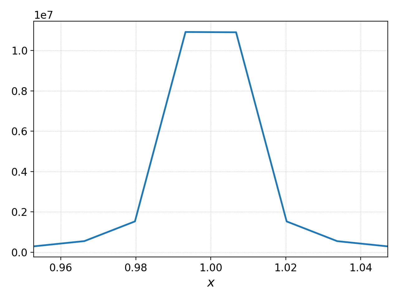
Ion heat flux to lower divertor at t=10 \(\mu\text{s}\)
Suppose instead of the instantaneous flux, we want the time-averaged flux over some period of time, perhaps from 5-10 \(\mu\text{s}\). To compute this, we can use
pgkyl "gk-sheath_ion_bcZlower_flux_Energy_*.bp" interp collect \
  sel --z0 5:10 ev 'f[0] 0,2,3 avg' pl -x '$x$'
This uses the collect command to aggregate the
frames into a time dimension, which becomes coordinate 0. We then use
sel --z0 5:10 to select frames 5-10. Then we use ev 'f[-1] 0,2,3 avg'
to average the data in the 0th (time), 2nd (\(y\)), and 3rd (\(z\))
dimensions. This gives
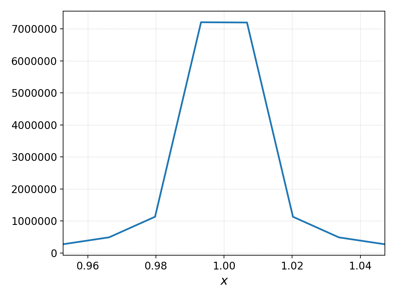
Time-averaged ion heat flux to lower divertor (t= 5-10 \(\mu\text{s}\))
References
Shi, E. L., Hammett, G. W., Stoltzfus-Dueck, T., & Hakim, A. (2019). “Full-f gyrokinetic simulation of turbulence in a helical open-field-line plasma”, Physics of Plasmas, 26, 012307. https://doi.org/10.1063/1.5074179