A first Gkeyll simulation
Gkeyll supports several models and numerous capabilities. Before diving into those, here’s a short overview of an input file, how to run it and plot its results.
Physics model
Consider the collisionless Landau damping of an electrostatic wave in a plasma. We simulate it with the Vlasov-Maxwell model:
More information about the model can be found in the Vlasov-Maxwell documentation. In this case we consider an electrostatic wave, and there are subtleties regarding electrostatic simulation using Maxwell’s induction equations. So we initialize the electron density as having a small sinusoidal perturbation:
and initialize the electric field in a manner consistent with the Poisson equation (using quasineutrality of the equilibrium electron and ion densities, \(n_i(x,t=0)=n_0\)):
Input file
This simulation is setup using Normalized units for the Vlasov-Maxwell system in a short Lua input file, which begins with the Preamble:
local Plasma = require("App.PlasmaOnCartGrid").VlasovMaxwell()

permitt  = 1.0   -- Permittivity of free space.
permeab  = 1.0   -- Permeability of free space.
eV       = 1.0   -- Elementary charge, or Joule-eV conversion factor.
elcMass  = 1.0   -- Electron mass.
ionMass  = 1.0   -- Ion mass.

nElc = 1.0    -- Electron number density.
nIon = nElc   -- Ion number density.
Te   = 1.0    -- Electron temperature.
Ti   = Te     -- Ion temperature.

vtElc   = math.sqrt(eV*Te/elcMass)                   -- Electron thermal speed.
vtIon   = math.sqrt(eV*Ti/ionMass)                   -- Ion thermal speed.
wpe     = math.sqrt((eV^2)*nElc/(permitt*elcMass))   -- Plasma frequency.
lambdaD = vtElc/wpe                                  -- Debye length.

-- Amplitude and wavenumber of sinusoidal perturbation.
pertA = 1.0e-3
pertK = .750/lambdaD

-- Maxwellian in (x,vx)-space, given the density (denU), bulk flow
-- velocity (flowU), mass and temperature (temp).
local function maxwellian1D(x, vx, den, flowU, mass, temp)
   local v2   = (vx - flowU)^2
   local vtSq = temp/mass
   return (den/math.sqrt(2*math.pi*vtSq))*math.exp(-v2/(2*vtSq))
end
The Preamble typically consists of a line loading the Gkeyll plasma ‘App’ to be used
(in this case VlasovMaxwell), and a specification of a number of user input parameters
and simple derived quantities. One can also create user-defined functions, like
maxwellian1D in this case, which may be used in the preamble or in the Gkeyll
App that follows. For this specific simulation the Gkeyll app is created by the following:
plasmaApp = Plasma.App {
   tEnd         = 20.0/wpe,           -- End time.
   nFrame       = 20,                 -- Number of output frames.
   lower        = {-math.pi/pertK},   -- Lower boundary of configuration space.
   upper        = { math.pi/pertK},   -- Upper boundary of configuration space.
   cells        = {64},               -- Configuration space cells.
   polyOrder    = 1,                  -- Polynomial order.
   periodicDirs = {1},                -- Periodic directions.

   elc = Plasma.Species {
      charge = -eV, mass = elcMass,
      lower = {-6.0*vtElc},      -- Velocity space lower boundary.
      upper = { 6.0*vtElc},      -- Velocity space upper boundary.
      cells = {64},              -- Number of cells in velocity space.
      init = function (t, xn)    -- Initial conditions.
         local x, v = xn[1], xn[2]
         return (1+pertA*math.cos(pertK*x))*maxwellian1D(x, v, nElc, 0.0, elcMass, Te)
      end,
      evolve = true, -- Evolve species?
   },

   ion = Plasma.Species {
      charge = eV, mass = ionMass,
      lower = {-6.0*vtIon},      -- Velocity space lower boundary.
      upper = { 6.0*vtIon},      -- Velocity space upper boundary.
      cells = {64},              -- Number of cells in velocity space.
      init  = function (t, xn)   -- Initial conditions.
         local x, v = xn[1], xn[2]
         return maxwellian1D(x, v, nIon, 0.0, ionMass, Ti)
      end,
      evolve = true, -- Evolve species?
   },

   field = Plasma.Field {
      epsilon0 = permitt, mu0 = permeab,
      init = function (t, xn)   -- Initial conditions.
         local Ex, Ey, Ez = -pertA*math.sin(pertK*xn[1])/pertK, 0.0, 0.0
         local Bx, By, Bz = 0.0, 0.0, 0.0
         return Ex, Ey, Ez, Bx, By, Bz
      end,
      evolve = true, -- Evolve field?
   },
}
The Gkeyll App typically consists of three sections:
Common: a declaration of parameters that control the (configuration space) discretization, and time advancement. This first block of code in
Plasma.Appmay specify the periodic directions, the MPI decomposition, and the frequency with which to output certain diagnostics.Species: Definition of the species to be considered in the simulation. Each species gets its own Lua table, in which one provides the velocity-space domain and discretization of that species (for kinetic models), initial condition, diagnostics, boundary conditions, and whether to evolve it or not (
evolve).Fields: A field table, which tells the App whether to evolve the electric and/or magnetic fields according to the field equations of the model. In this table we also specify the initial condition of the fields.
In some applications other sections of the Plasma.App may be necessary, for example, to specify the geometry.
Finally, an input file concludes with an invocation of the App’s run method:
plasmaApp:run()
Running your first simulation
Now that we have a Gkeyll input file (named vm-damp.lua),
simply run the simulation by typing
gkyl vm-damp.lua
You should see the program printing to screen like this:
wsName:gkyldir gabriel$ gkyl vm-damp.lua
Tue Sep 15 2020 16:16:44.000000000
Gkyl built with b0b8203670c7+
Gkyl built on Sep 14 2020 16:29:40
Initializing PlasmaOnCartGrid simulation ...
 ** WARNING: timeStepper not specified, assuming rk3
Using CFL number 0.333333
Initializing completed in 0.0629927 sec

Starting main loop of PlasmaOnCartGrid simulation ...

 Step 0 at time 0. Time step 0.00727108. Completed 0%
0123456789 Step   276 at time 2.00698. Time step 0.00727174. Completed 10%
0123456789 Step   551 at time 4.00677. Time step 0.00727214. Completed 20%
0123456
Gkeyll prints a number every 1% of the simulation, and a longer message with the total number of time steps taken, the simulation time and the latest time step size every 10% of the simulation. This particular simulation ran in 74 seconds on a 2015 MacBookPro. As it progressed it wrote out diagnostic files.
Plotting
In this case we did not request additional diagnostics, so the only ones provided are default ones:
Distribution functions:
vm-damp_elc_#.bpandvm-damp_ion_#.bp.Electromagnetic fields:
vm-damp_field_#.bp.Field energy:
vm-damp_fieldEnergy.bp.
Fields that are larger (in memory) like the distribution function, get written out
periodically, not every time step. These snapshots (frames) are labeled by the number
# at the end of the file name.
In order to plot the initial distribution function of the electrons we will use the
Gkeyll post-processing tool (postgkyl), invoked by the pgkyl
command as follows
pgkyl vm-damp_elc_0.bp interpolate plot
This produces the 2D plot of the initial Maxwellian distribution given below.
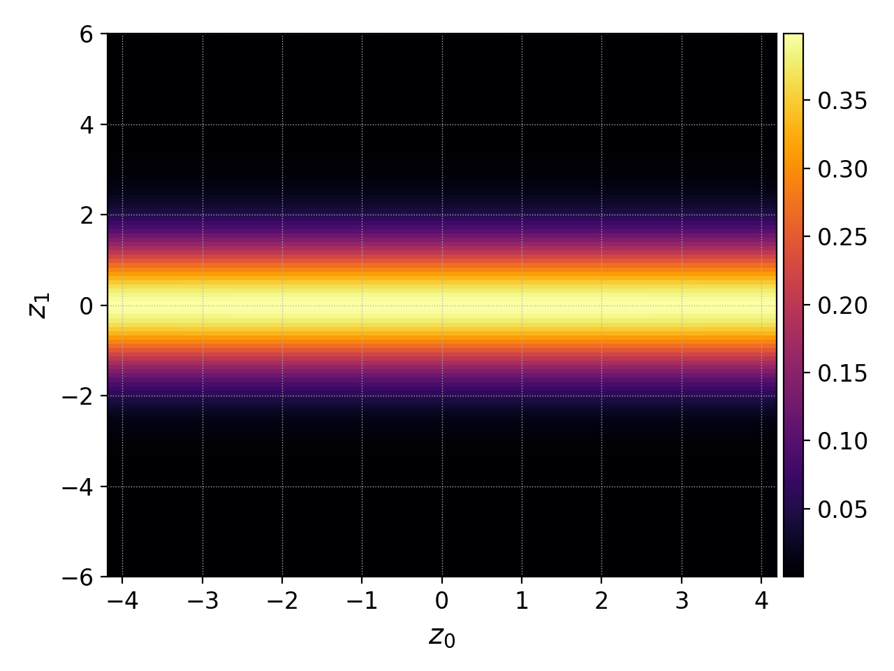
Initial electron distribution function, \(f_e(x,v,t=0)\).
We can also examine the electrostatic energy in the simulation. This most clearly
exhibits the wave energy decaying as the collisionless damping takes effect. For
this purpose we use the following postgkyl command (we select the
x-component, and pg_cmd-plot can use a log scale, as well as add labels):
pgkyl vm-damp_fieldEnergy.bp select -c0 plot --logy -x 'time' -y '$|E_x|^2$'
resulting in the following figure of the (normalized) electrostatic energy as a function of time
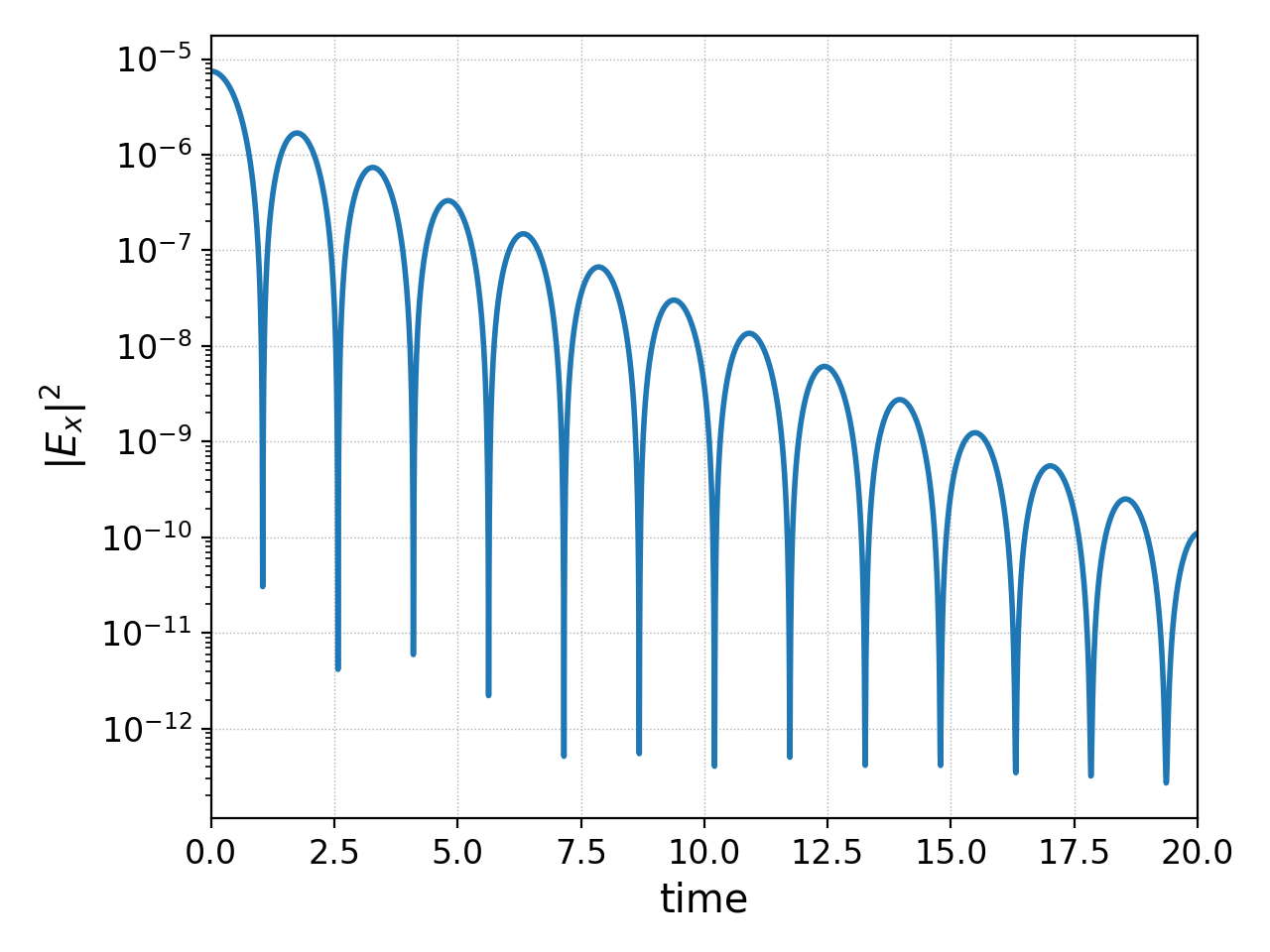
Normalized electrostatic field energy \(\propto |E_x|^2\) as a function of time (normalized to \(\omega_{pe}\)).
Additional quick-start examples
The above example used a Vlasov-Maxwell simulation to showcase how to setup, run and postprocess a Gkeyll simulation. In addition to Vlasov-Maxwell there are also Gyrokinetic and (fluid) Moment models. Each of these have slightly different features and ways of using them. Quick examples for each of these are found below: