ev
ev is a special command that enables simple operations like adding
or multiplying datasets directly in a terminal. As these operations
are generally simple to do in a script mode, ev is available only
in the command line interface.
Reverse Polish notation
ev uses reverse Polish notation (RPN; also know as postfix
notation) to input operations. Unlike in the more common infix
notation, in RPN, the operators follow operands. For example 4 - 2
is written in RPN as 4 2 -; 4 - (2 / 5) is 4 2 5 / -. This
can be further demonstrated on the sequence that processes this
expression.
4>>>4(Add 4 to the stack)4 2>>>4 2(Add 2 to the stack)4 2 5>>>4 2 5(Add 5 to the stack)4 2 5 />>>4 0.4(Divide the last two elements with each other)4 2 5 / ->>>3.6(Subtract the last two elements from each other)
More information about RPN can be found, for example, on Wikipedia.
Using ev on simple datasets
The ev command has one required argument, which is the operation
sequence. Datasets are specified in the sequence with
f[set_index][component]. Note that Python indexing conventions are
used. Specifically, when no indices are specified, everything is used,
i.e., f[0][:] and f[0] are treated as identical calls. The
indices need to be integers unless a global indexing mode -g is
used, which ignores active and inactive sets. Then, Python
slice syntax can be used as well including negative indices and
strides. For example, f[2:-1:2] will select every other dataset,
starting with the third one (zero-indexed), and ending with one before
the last (by Python conventions, the upper bound is not included; in
this example it might end with the third element from the end because
of the stride).
Note
Dataset selection in ev internally uses the same code as the
activate/deactivate/pg_cmd_deactivate commands, so the
following commands produce similar results (ev actually copies
the datasets instead of just activating some).
pgkyl two-stream_elc_?.bp activate -i '2:-1:2'
pgkyl two-stream_elc_?.bp ev -g 'f[2:-1:2]'
However, this is probably a fringe application of ev.
The simplest example of ev is a numerical operation performed on
a dataset, e.g., dividing the values by the insidious factor of 2:
pgkyl two-stream_elc_0.bp ev 'f[0] 2 /'
This can be also combined with the fact that ev can access dataset
metadata as long as they are included (which is a new feature in
Gkeyll introduced in January 2021). An example of this can be plotting
number density from a fluid simulation (Gkeyll outputs mass density).
pgkyl 5m_fluid_elc_0.bp ev 'f[0][0] f[0].mass /' plot
Note that on top of dividing by mass, only the first component, which corresponds to density, was selected. This can be easily extended to apply on multiple datasets and create an animation using the animate command
pgkyl '5m_fluid_elc_[0-9]*.bp' ev -g 'f[:][0] f[:].mass /' animate
The capabilities are not limited to operations with float factors. As
an example, ev can be used to visualize differences
(--diverging mode of the plot command is well suited
for this)
pgkyl two-stream_elc_0.bp two-stream_elc_80.bp interpolate ev 'f[1] f[0] -' plot --diverging
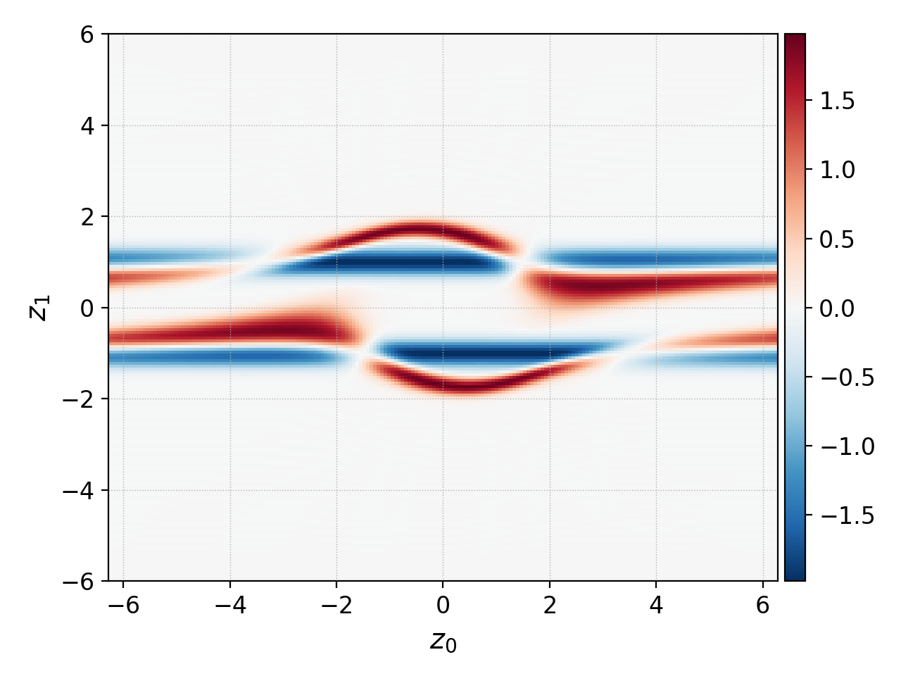
Visualizing the difference between two datasets
Note
info command, especially with the --compact
-c flag can be useful to print indices for available datasets.
The same concept can be used to calculate bulk velocity from the first two moments:
pgkyl two-stream_elc_M0_0.bp two-stream_elc_M1i_0.bp interpolate ev 'f[1] f[0] /' plot
Finally, it is worth noting that this syntax cannot be used when there are datasets with more than one tag active.
Using ev on datasets with tags
The ev command is tag-aware. Tagged datasets use the following
notation tag_name[set_index][component]. Using this, the
previous example can be reproduced:
pgkyl two-stream_elc_M0_0.bp -t dens two-stream_elc_M1i_0.bp -t mom interp ev 'mom dens /' plot
This can be naturally extended for batch loading and animate:
pgkyl 'two-stream_elc_M0_[0-9]*.bp' -t dens 'two-stream_elc_M1i_[0-9]*.bp' -t mom interp ev 'mom dens /' animate
Examples of specific ev operations
In this section we provide examples of some ev operations that
are less trivial or intuitive.
grad
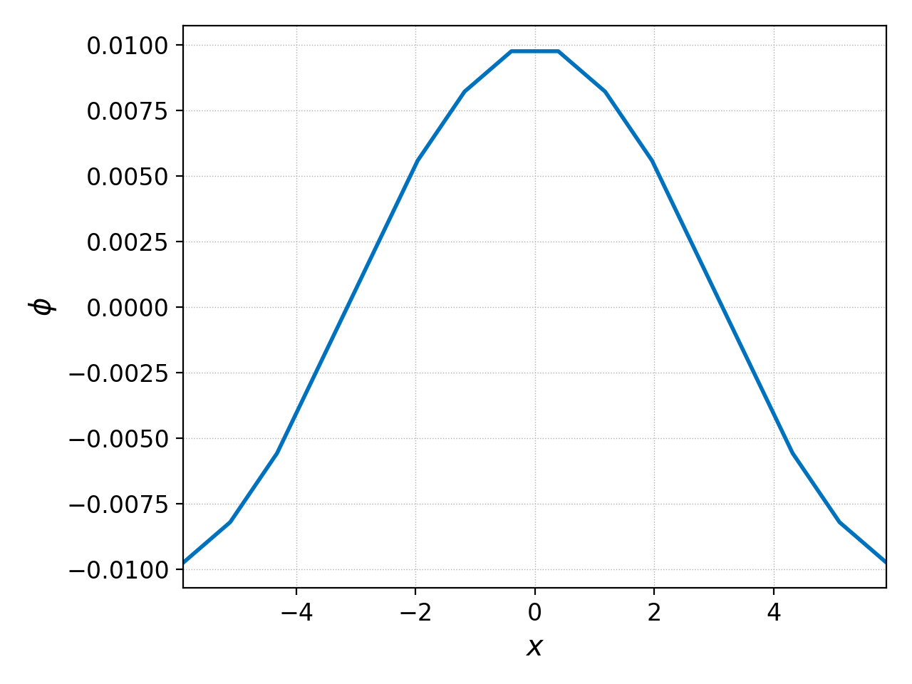
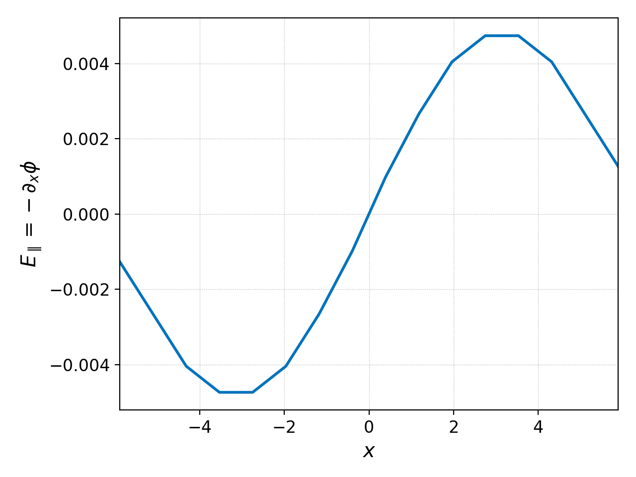
This operation differentiates a along a direction given by the second operand. So, for example, given the data from an ion sound wave gyrokinetic simulation we can plot the initial electrostatic potential with
pgkyl gk-ionSound-1x2v-p1_phi_0.bp interp pl -x '$x$' -y '$\phi$'
and compute the parallel electric field by differentiating the potential along \(x\) as follows:
pgkyl gk-ionSound-1x2v-p1_phi_0.bp interp ev 'f[0] 0 grad -1 *' pl -x '$x$' -y '$\phi$'
These produce the following plots:
int
Integrate a dataset along a direction specified by the second operand,
or along multiple directions specified by a comma-separated list. If we
once again take the
ion sound wave gyrokinetic simulation
data, we can examine the number of particles in the simulation (should be
conserved) by taking the time trace of the integrated ion number density
(intM0) and taking its mean:
pgkyl gk-ionSound-1x2v-p1_ion_intM0.bp ev 'f[0] mean' pr
which prints out
12.566370614358858
If we instead use ev to integrate the initial and/or the final number
density GkM0, we should get roughly the same answer. We can check that
this is the case by typing
pgkyl gk-ionSound-1x2v-p1_ion_GkM0_10.bp interp ev 'f[0] 0 int' pr
which produces
12.566370614358522
and we have shown that the number of particles at the end is roughly the same as the mean number of particles throughout the simulation.
avg
Average a dataset along a direction specified by the second operand, or along multiple directions specified by a comma-separated list.