integrate¶

Integrate a dataset over specified direction(s).

Command line¶

$ pgkyl integrate --help
  Usage: pgkyl integr [OPTIONS] AXIS

    Integrate data over a specified axis or axes

  Options:
    -u, --use TEXT  Specify the tag to integrate
    -t, --tag TEXT  Optional tag for the resulting array
    -h, --help      Show this message and exit.

Consider the gyrokinetic simulation of an ion acoustic wave as an example. It outputs the integrated particle density over time, which can plot as follows:

pgkyl gk-ionSound-1x2v-p1_ion_intM0.bp pl

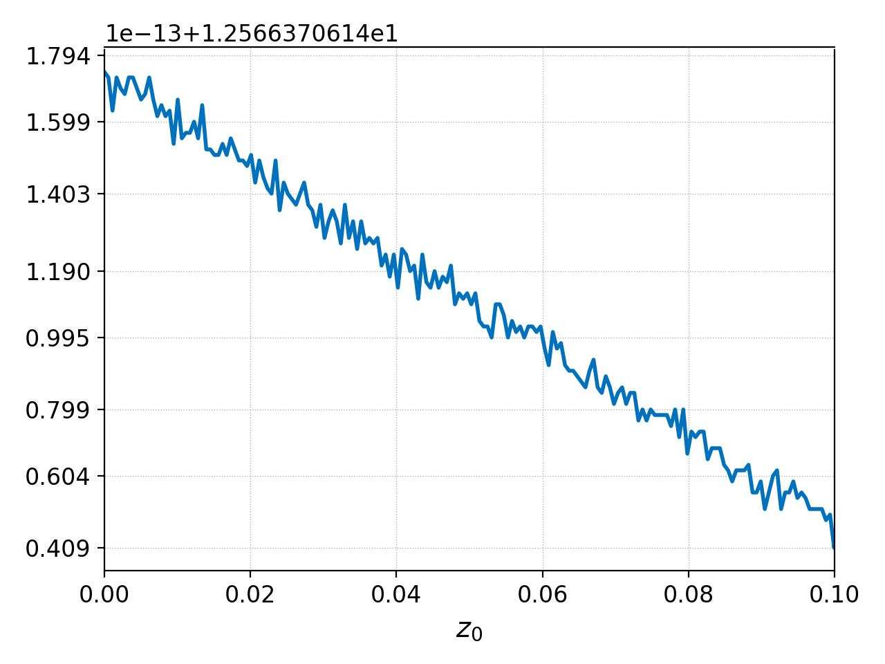
../../_images/gk-ionSound-1x2v-p1_intM0.png

We can see from the values on the y-axis that the total number of particles is 12.566. The number of particles should be conserved, to machine precision. We can check this another way by integrating the particle density along \(x\) (the 0th dimension) at the end of the simulation with pgkyl:

pgkyl gk-ionSound-1x2v-p1_ion_GkM0_1.bp interp integr 0 print

where we have abbreviated integrate with integr, and we use the print command to print the result of the integral to screen. The output of this command is simply

12.566370614359034

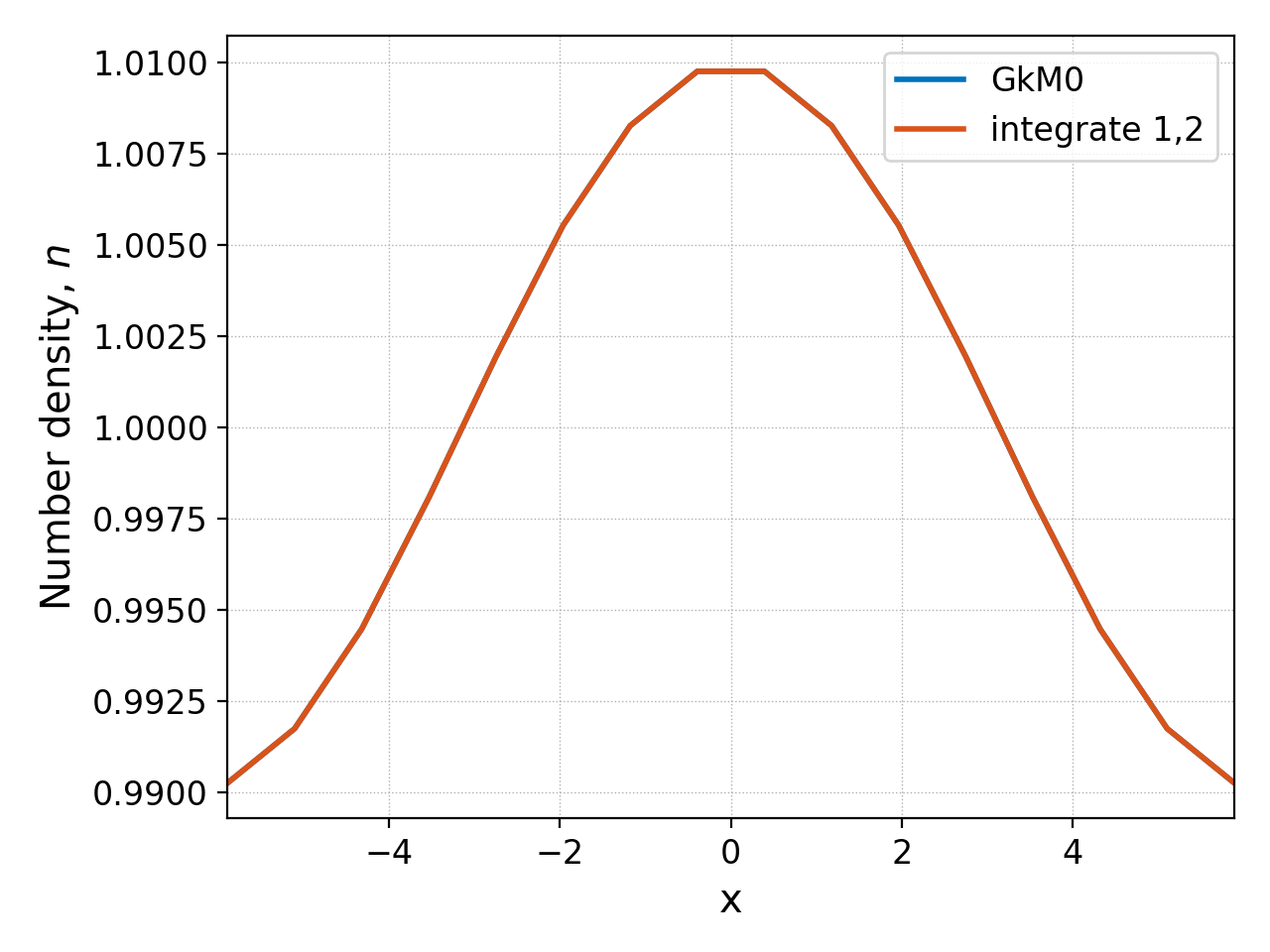
The integrate command can also be used to integrate higher dimensional datasets in one or more directions. We could take the ion distribution function and integrated along the \(v_\parallel\) and \(\mu\) directions (1st and 2nd dimensions, respectively) with

pgkyl gk-ionSound-1x2v-p1_ion_0.bp gk-ionSound-1x2v-p1_ion_GkM0_0.bp interp \
  activate -i 0 integr 1,2 ev -l 'integrate 1,2' 'f[0] 6.283185 *' \
  activate -i1,2 pl -f0 -x 'x' -y 'Number density, $n$'

Note

In this command we:

First load the ion distribution function (*_ion_0.bp) and its number density (*_ion_GkM0_0.bp) at \(t=0\).
Integrate the distribution function over velocity space with activate -i 0 integr 1,2.
Multiply such integral by \(2\pi B_0/m_i\) (\(B_0=m_i=1\) here) with ev -l 'integrate 1,2' 'f[0] 6.283185 *'.
Activate the number denstiy and integrated distribution function data sets and plot them with activate -i1,2 pl -f0.

and this should give approximately the same number density as the GkM0 diagnostic outputted by the simulation, as shown below.

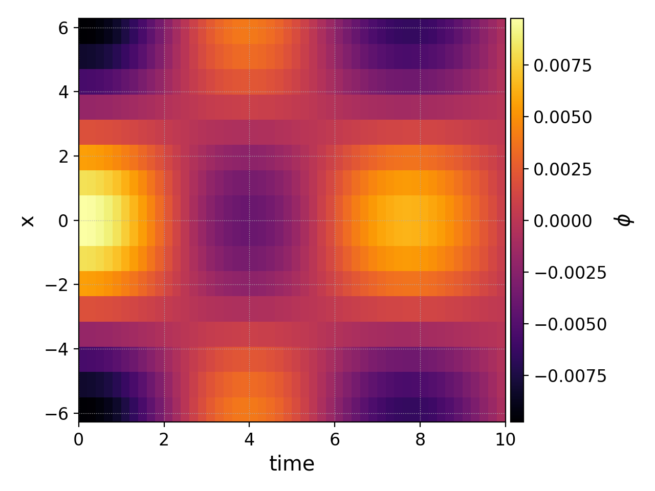
../../_images/gk-ionSound-1x2v-p1_ion_GkM0_0.png

Another useful application of the integrate command is to integrate, or average, over time (although note that the ev command has a avg operation that may make this easier). Usually this requires collecting multiple frames into a single dataset with the collect command, and then integrating over the 0th dimension (time).

So if we increase the tEnd of the gyrokinetic ion sound wave simulation to 10 and the number of frames to 50 we could plot the electrostatic potential as a function of time and position with

pgkyl "gk-ionSound-1x2v-p1_phi_[0-9]*.bp" interp collect pl -x 'time' -y 'x' --clabel '$\phi$'

../../_images/gk-ionSound-1x2v-p1_phi.png

We can integrate this potential in time and plot it on top of the initial potential with

pgkyl gk-ionSound-1x2v-p1_phi_0.bp -l '$t=0$' -t phi0 \
  "gk-ionSound-1x2v-p1_phi_[0-9]*.bp" -t phis interp collect -u phis -t phiC \
  integrate -u phiC -t phiInt 0 ev -l 'Time average' -t phiAvg 'phiInt 10. /' \
  activate -t phi0,phiAvg pl -f0 -x '$x$' -y '$\phi$'

This command uses tags to select which dataset to perform an operation on. The end result is the plot below

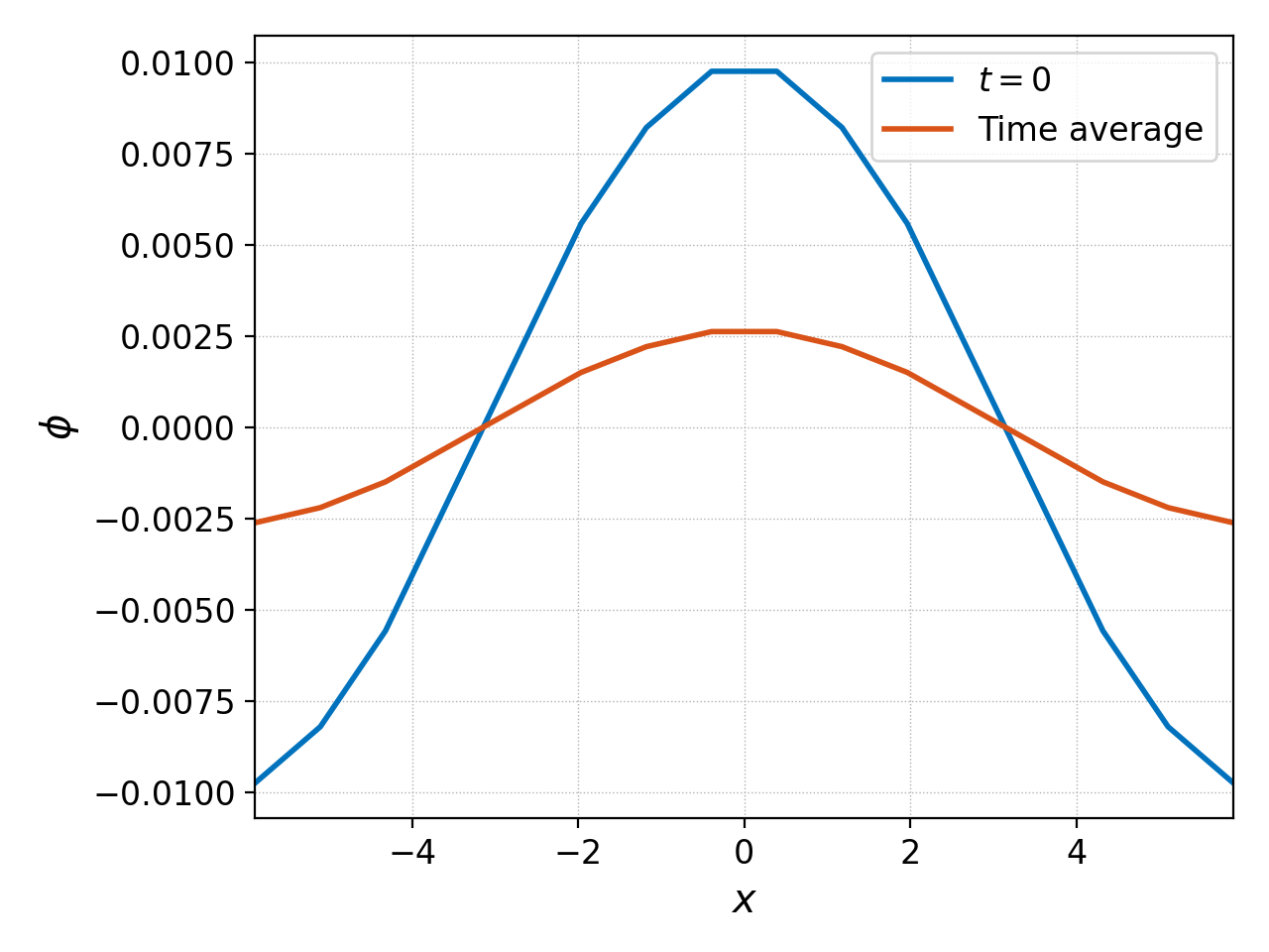
../../_images/gk-ionSound-1x2v-p1_phi_0_tAv.png

showing that the time averaged potential is lower amplitude due to the collisionless Landau damping of the wave.